This AAPL trading strategy would have given a return of $31,712,009 for every dollar invested in December 1980. That's 123,000 times better than buy-hold, with nearly four times the annualized return (61.4% vs 16.7% for buy-hold) and roughly half the drawdown which amounts to over six times better reward/risk than buy-hold.
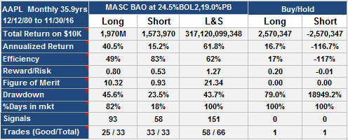
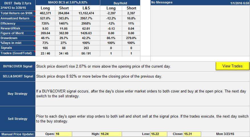
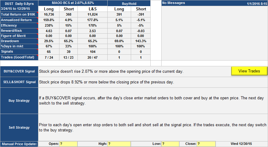
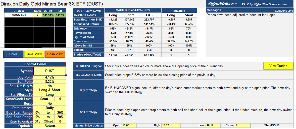
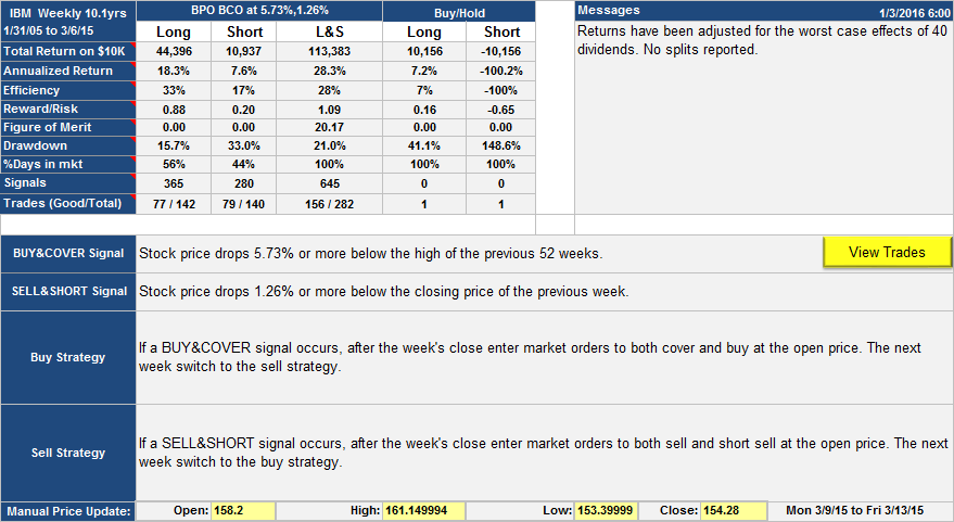
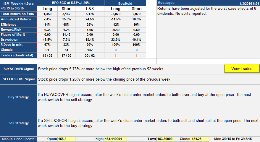
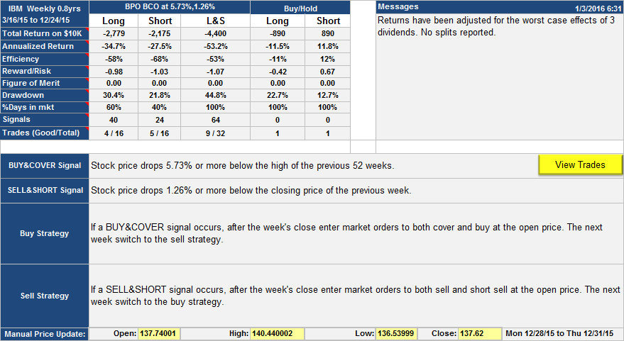
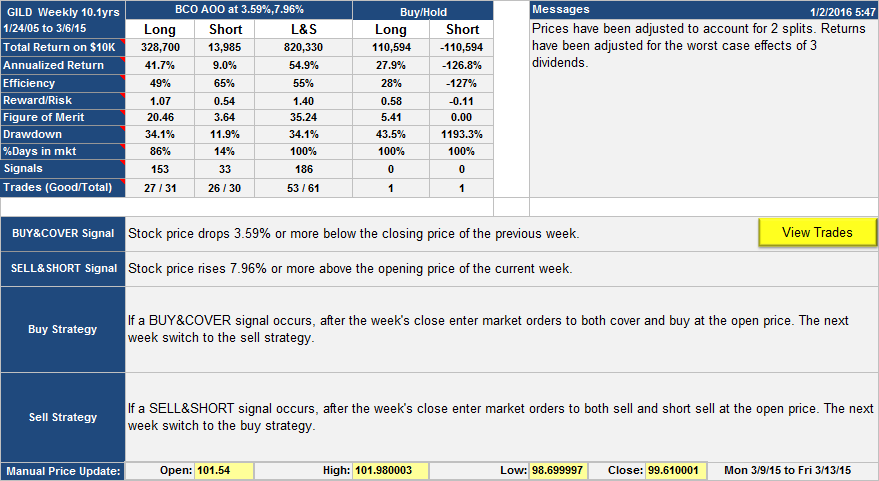
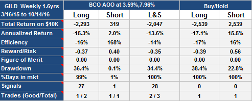
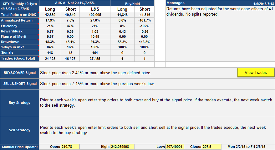
AAPL $31,000,000 trading strategy: Table of results
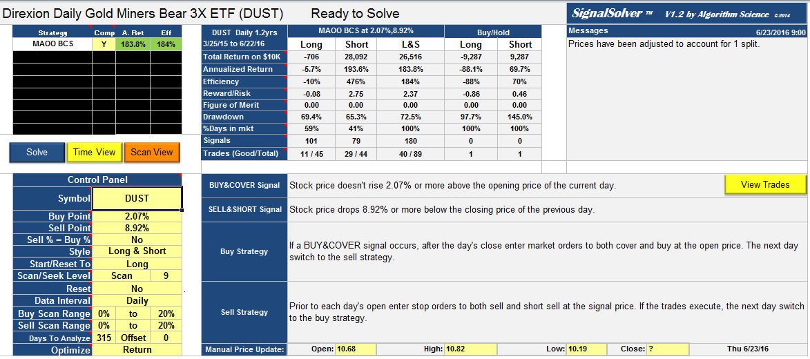
This is a variation of the MASC BAO algorithm which I have published before, except this time the buy point is related to a Bollinger Band instead of just the sell price. I found it using SignalSolver.
Here is the strategy:
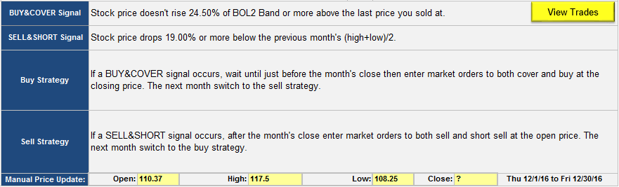
Description of the AAPL $31,000,000 trading strategy
In this case the Bollinger band is the 7 period StdDev of median prices (monthly (H+L)/2), and the band is built around the last sell price, not the usual method of building it around a moving average. A little unconventional but it worked wonderfully. Algorithms with buy signals based on sell price often get stuck, but this one didn't. Sell signals were based on a raw Percentage Band built around the monthly median (H+L)/2 prices, just like the original version of this.
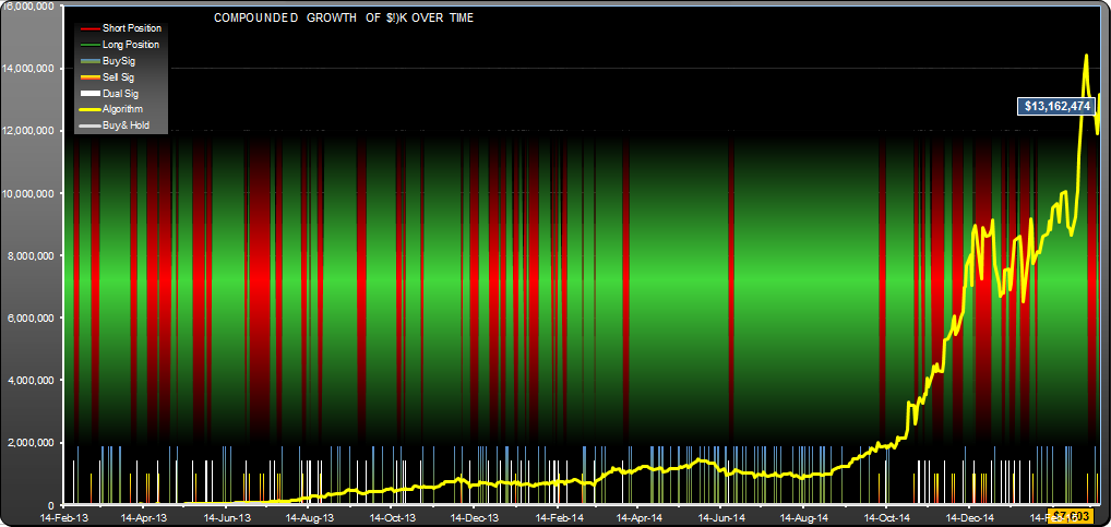
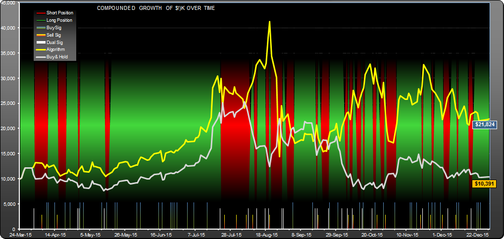
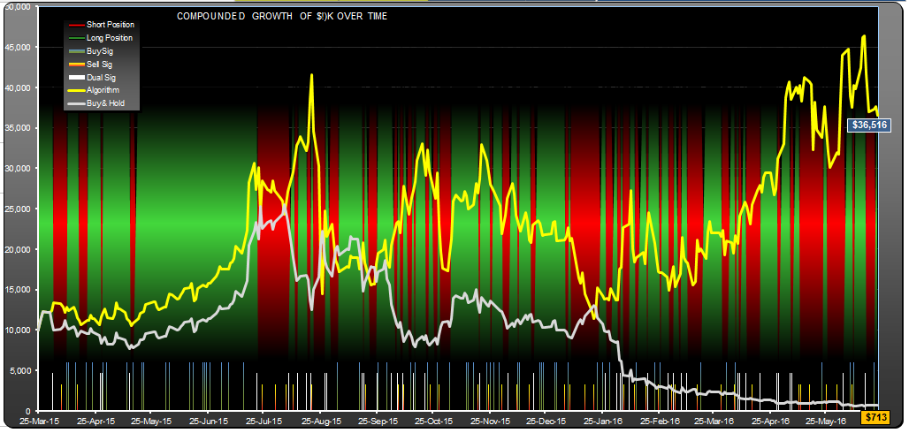
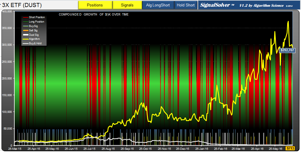
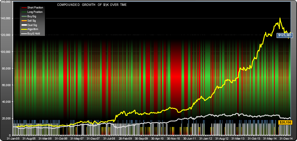
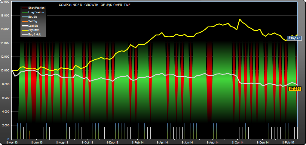
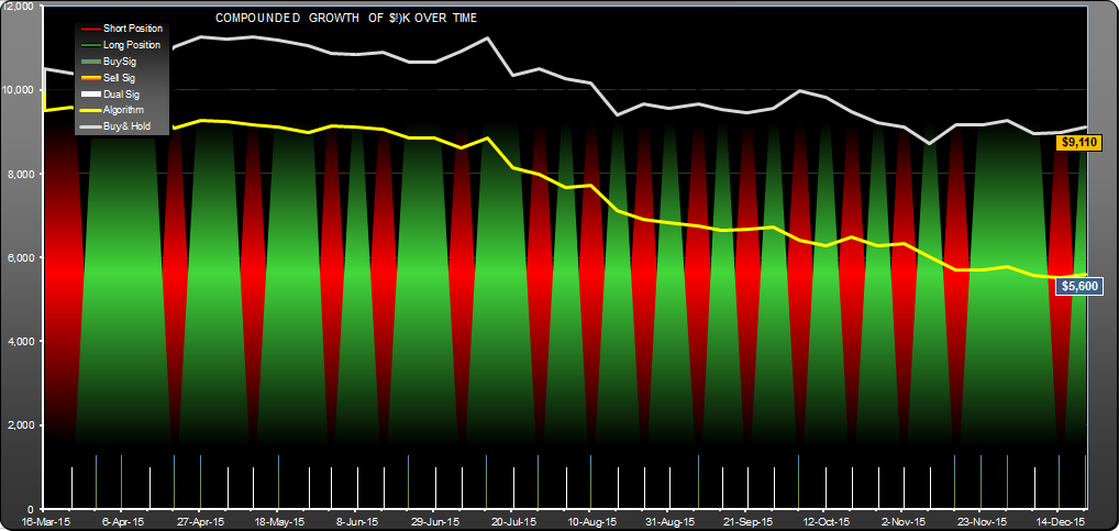
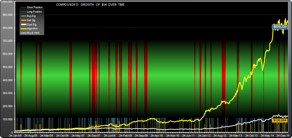
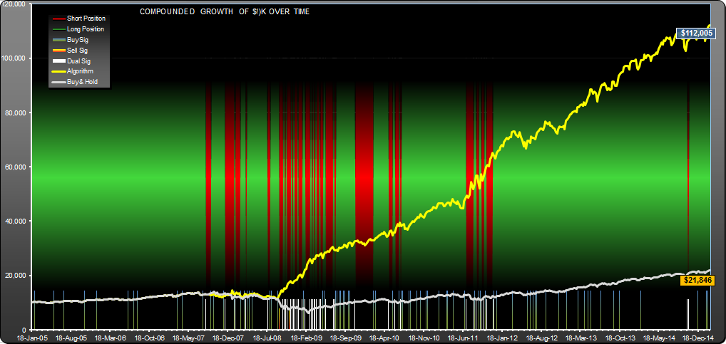
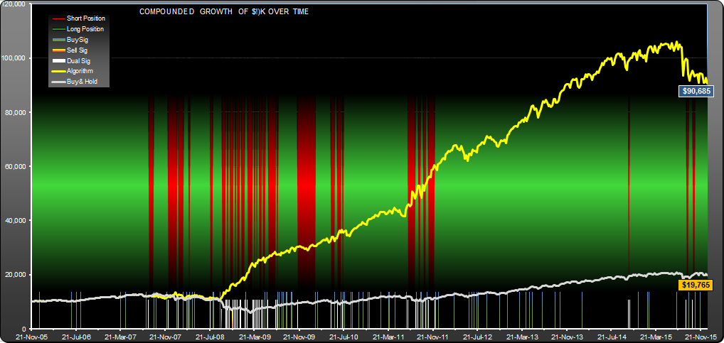
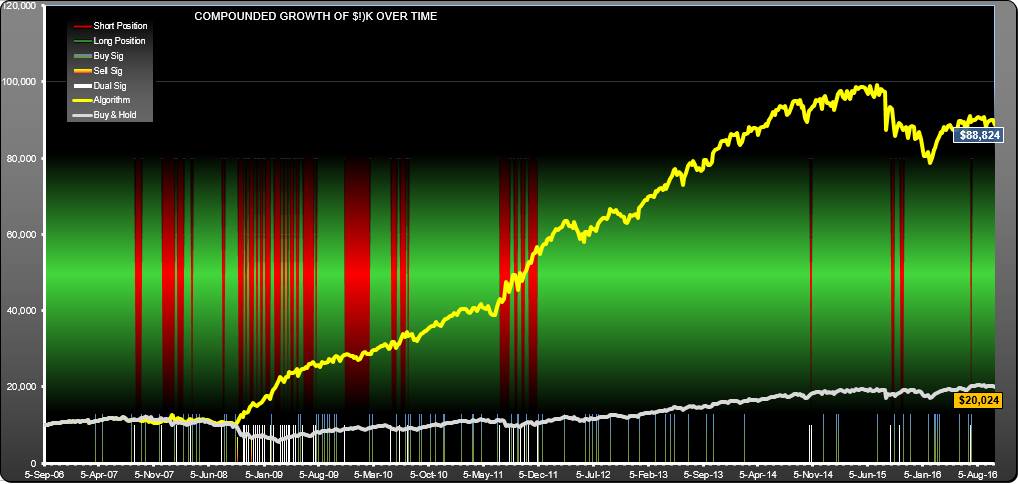
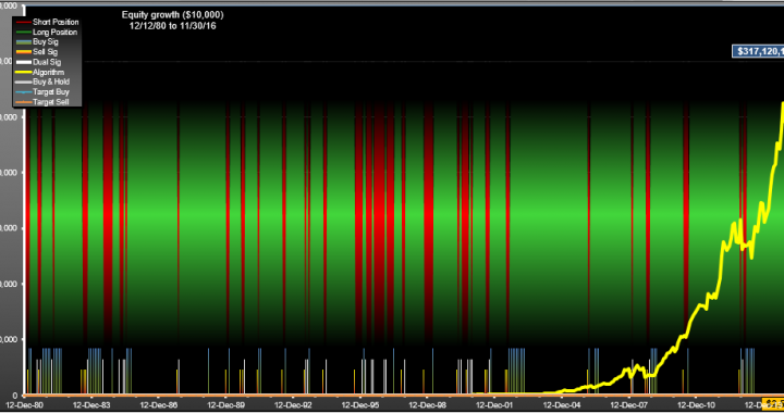
Here is the equity curve:
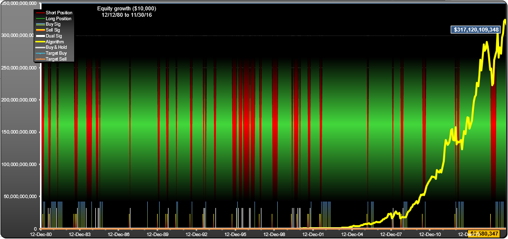
We are looking at quite a bit of reinforcement on buy signals, but sell signals tend to come in ones or twos. There are some dual signal months but not too many. Dual signals will trigger a trade for this algorithm.
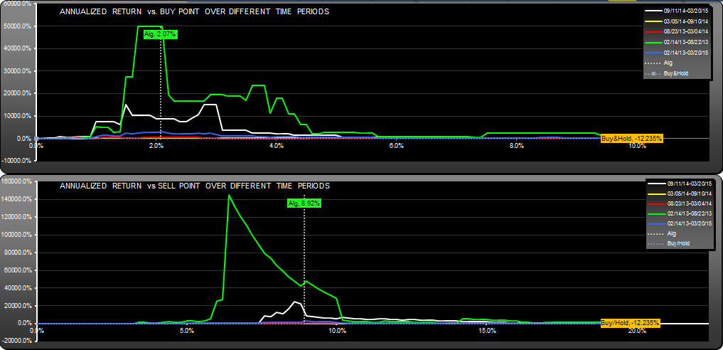
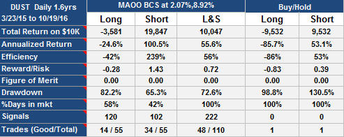
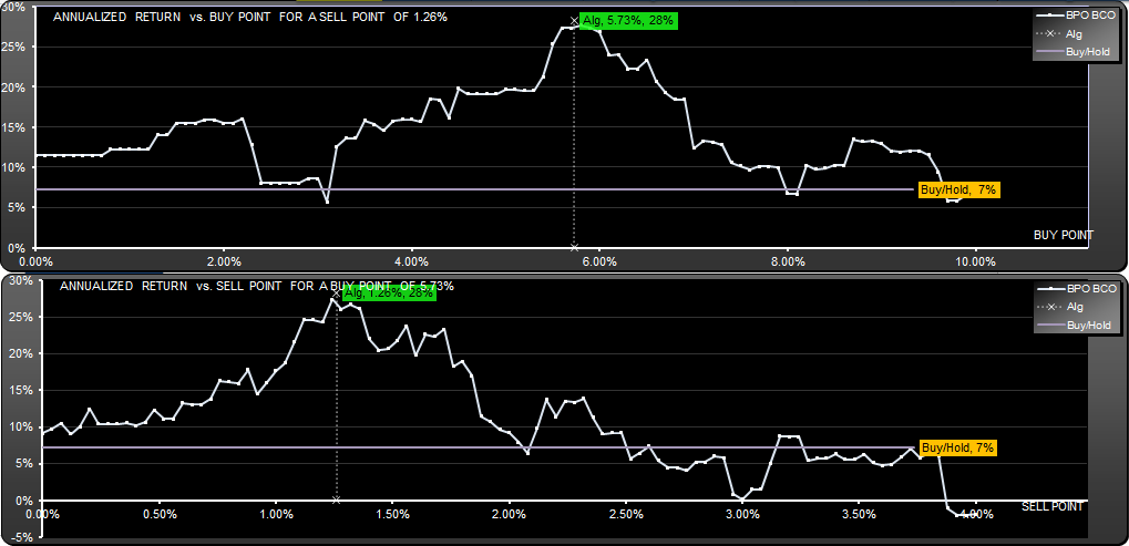
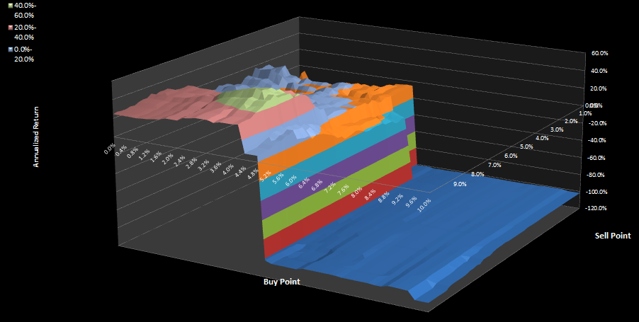
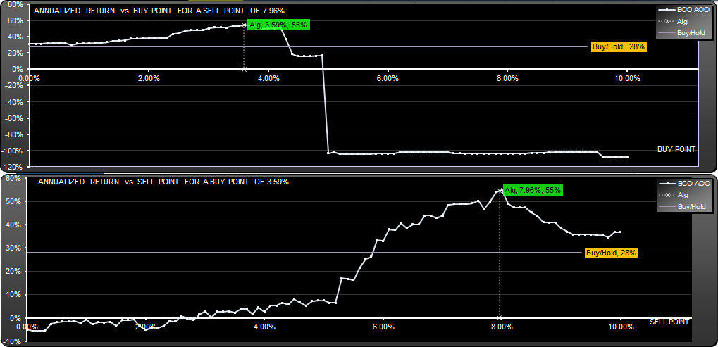
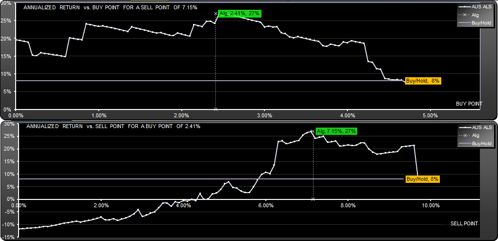
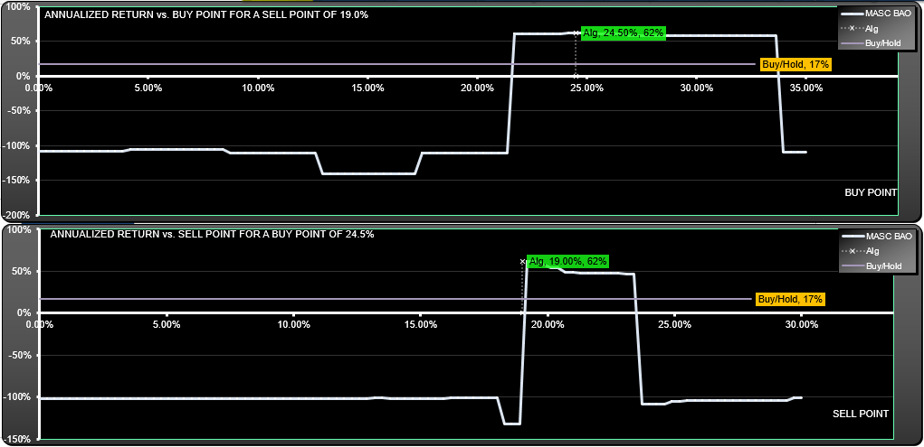
Moving onto the scans, you can see that there is a single area of profitability:
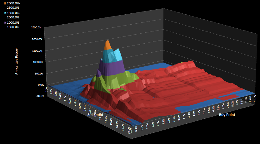
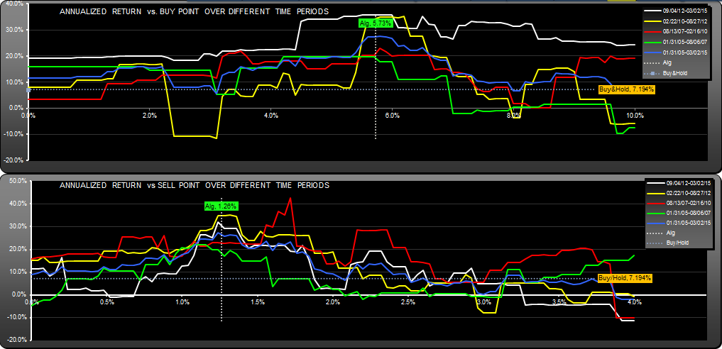
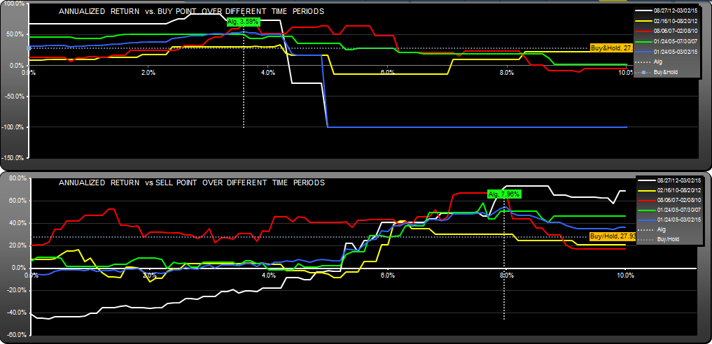
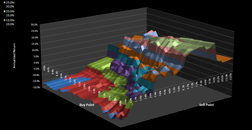
Getting the buy or especially the sell point wrong would have led to a complete loss, as this algorithm was run Long and Short (you were either long or short at all times). Here's the entire parameter surface, for completeness:
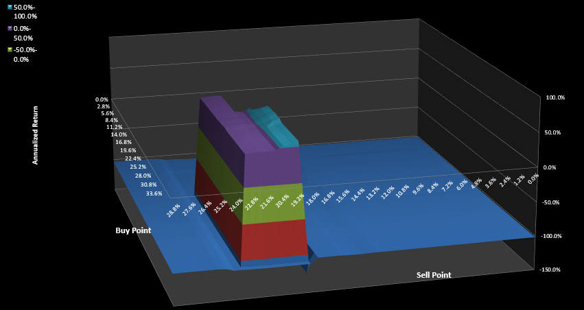
A bit of a steep sided mesa, but a reasonably large plateau.
Since I found it in June, the algorithm has added about 3%, but it hasn't traded and is still long.
Here are the trades: AAPL.M4 List of trades
AAPL MASC BAO Update Aug 4th 2017
The algorithm has added around 40% since publication in Dec 2016, return on $10K would now be $432,155,847,777 . There have been no signals or trades and the position remains long.
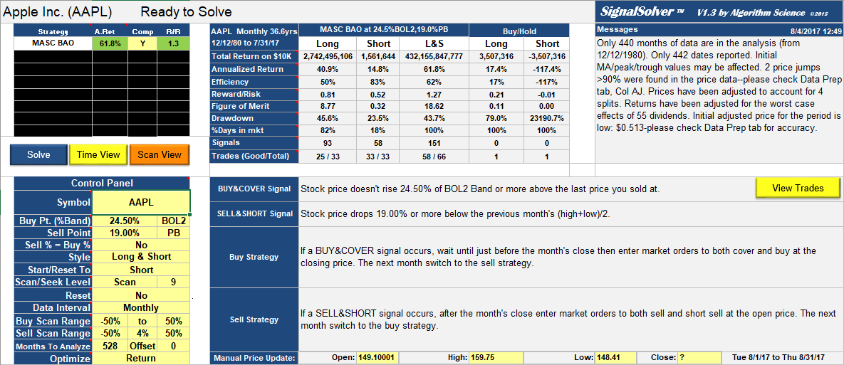
AAPL Monthly Trading Algorithm MASC BAO $432,155,847,777 return for $10K initial investment, update 8/4/2017