AAPL Trading System (Monthly)

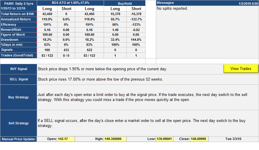
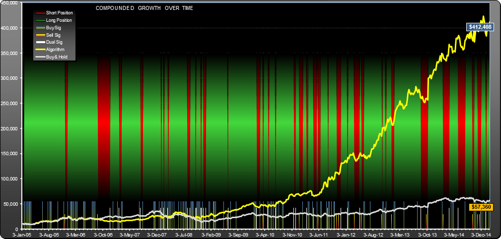
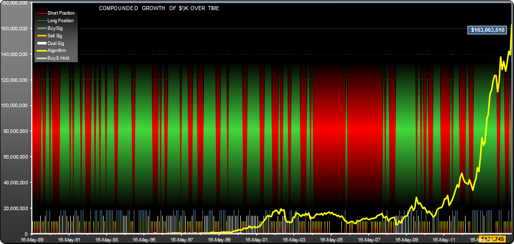
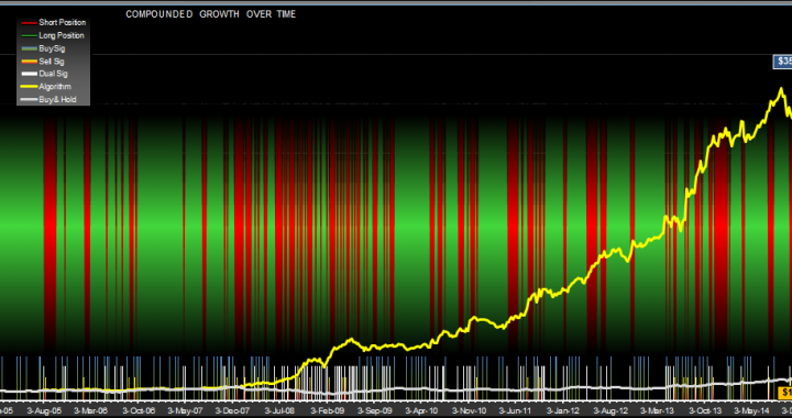
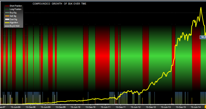
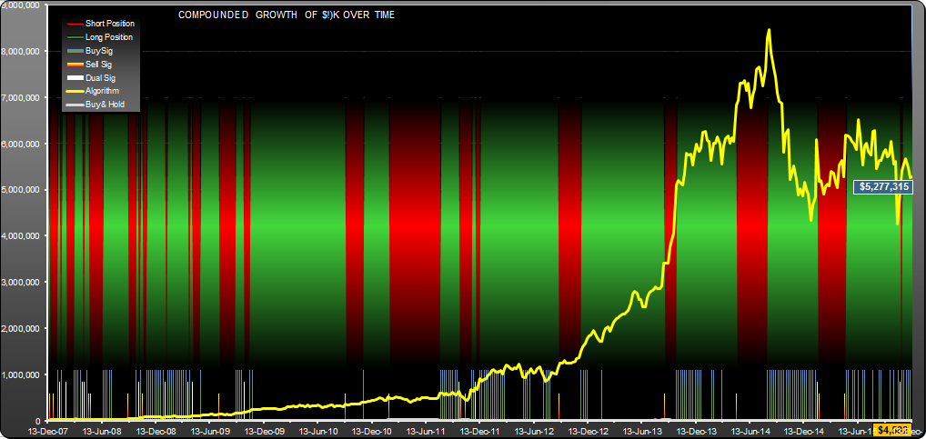
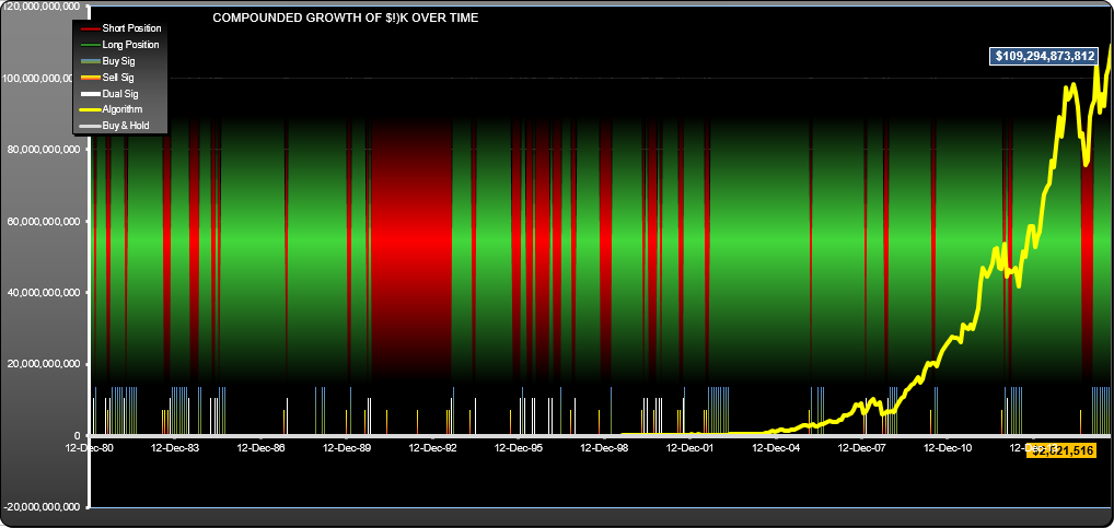
With $94 billion in profits (for $10K initial investment) this has one of the highest total returns I have seen for any algorithm.

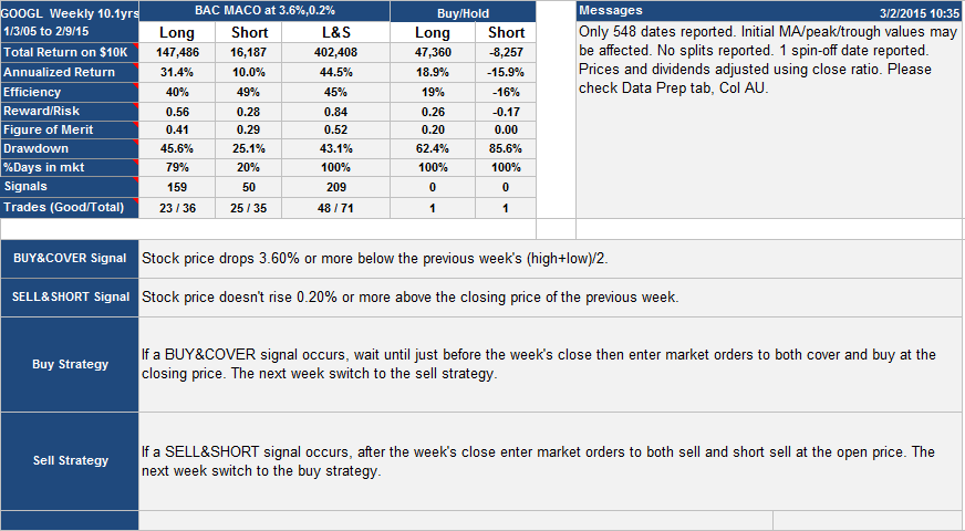
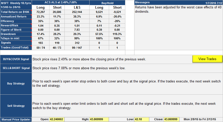
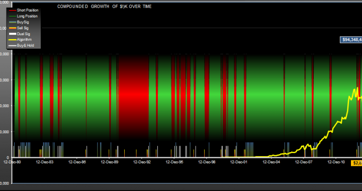
It is an interesting study, but I wouldn't recommend it as a good system to trade moving forward. It is somewhat over-tuned, and the parameters are close to regions which would have failed. At one time the equity went negative and you would have required extra capital to satisfy margin calls. The algorithm uses the "last sell price" as a reference. This can lock up an algorithm if the stock price is trending, in this case starving it of buy signals if the buy and sell percentages were chosen wrongly.

That said, I've been watching it for a year or so and it has behaved itself. The one take-away that you might find valuable--if you are holding AAPL and you see that portentous 19.44% or more price drop in a month, maybe you should take heed and sell at the next monthly open. The 29 times this happened over the last 34 years, you could buy at a better price later on.

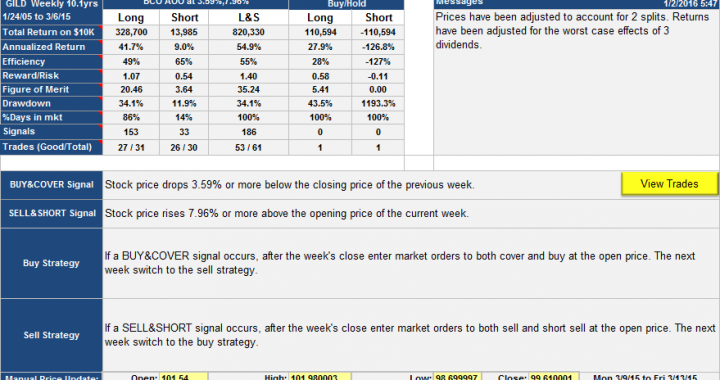
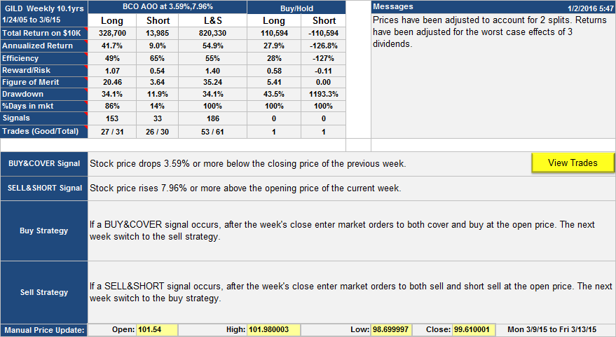
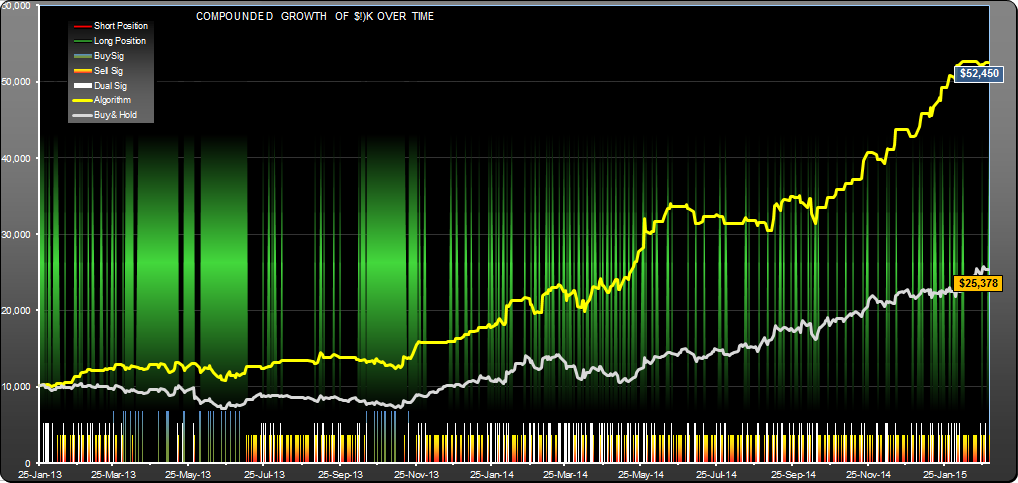
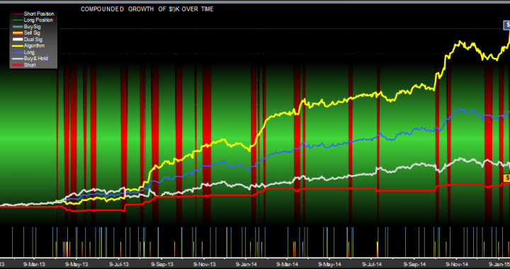
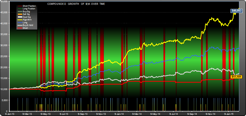
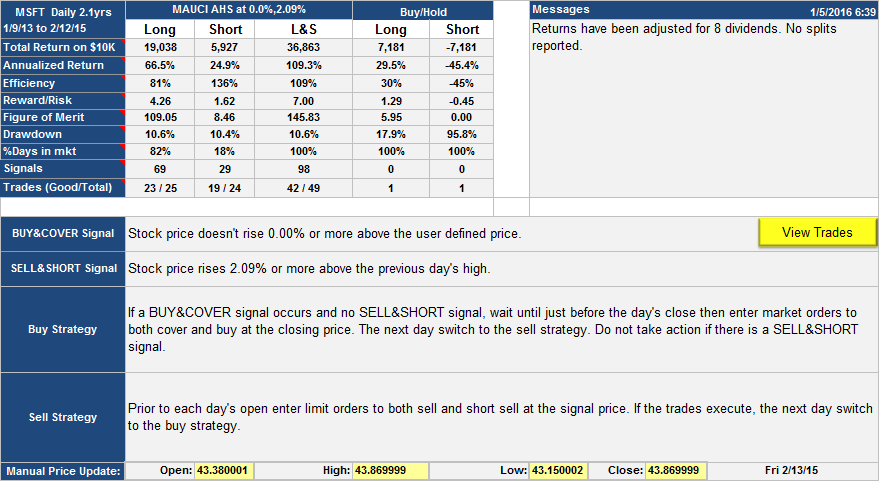
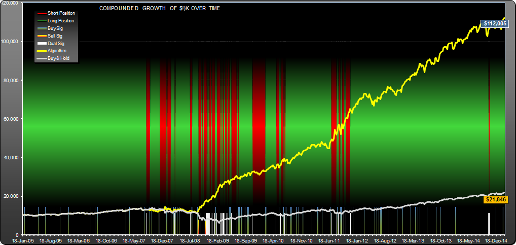
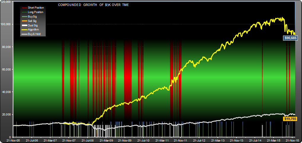
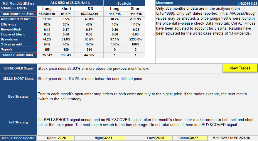
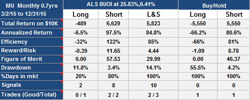
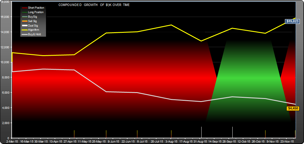
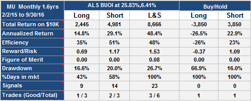
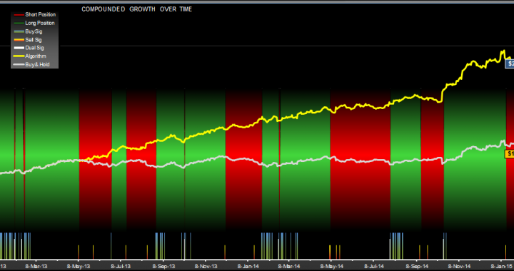
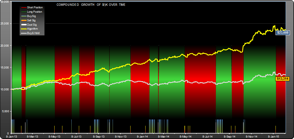
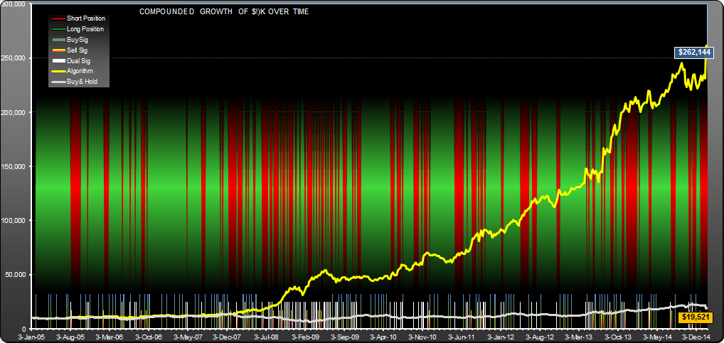
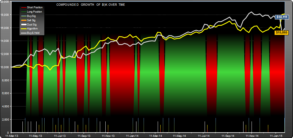
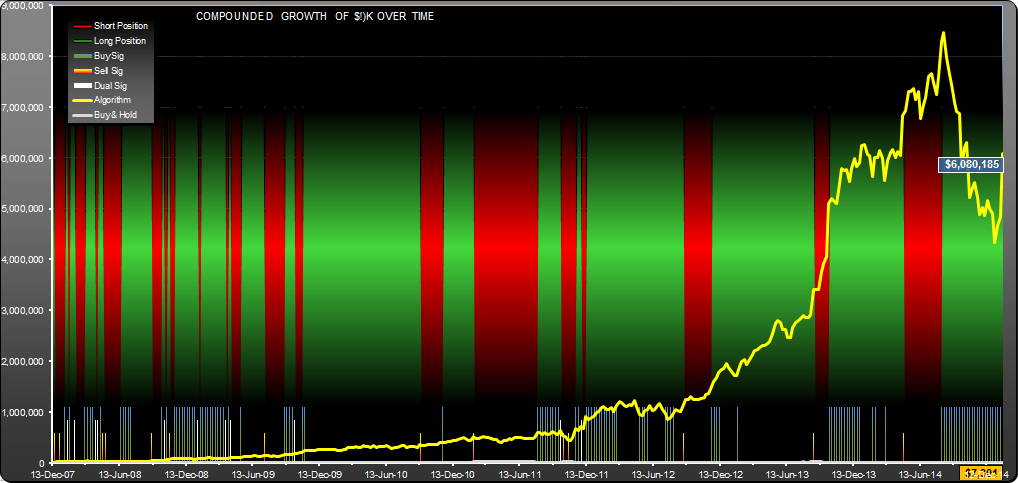
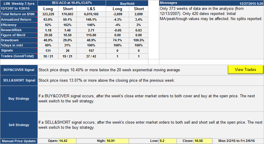
Notes: returns are compounded, commission was $7 per trade. Here is a list of trades: AAPL.M Trades

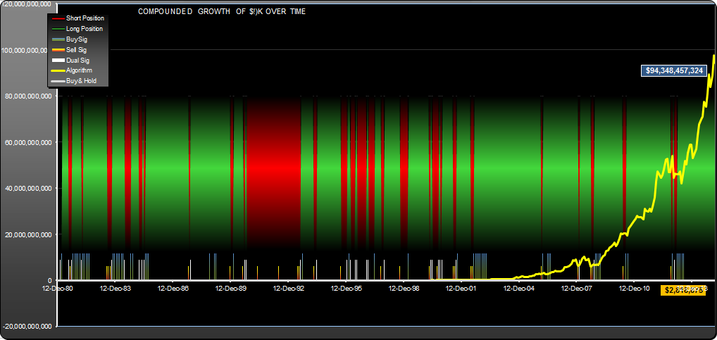
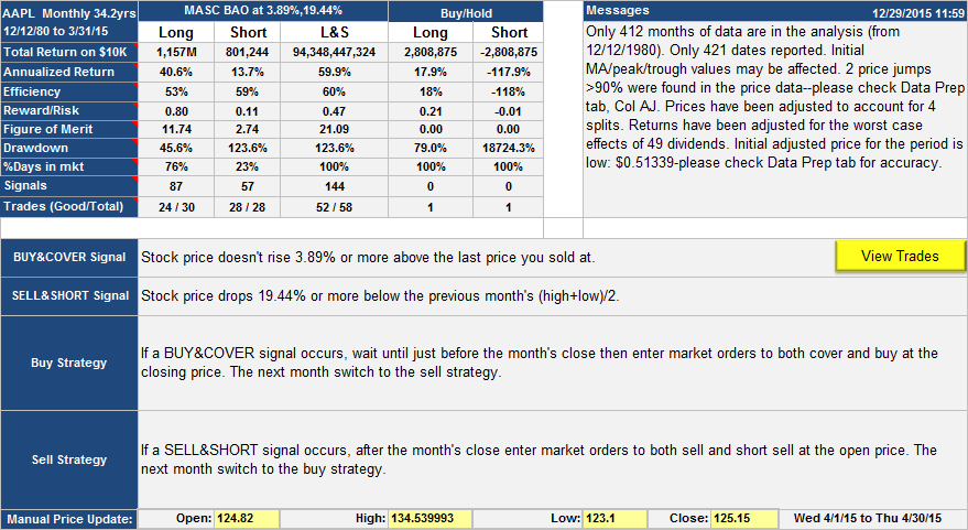
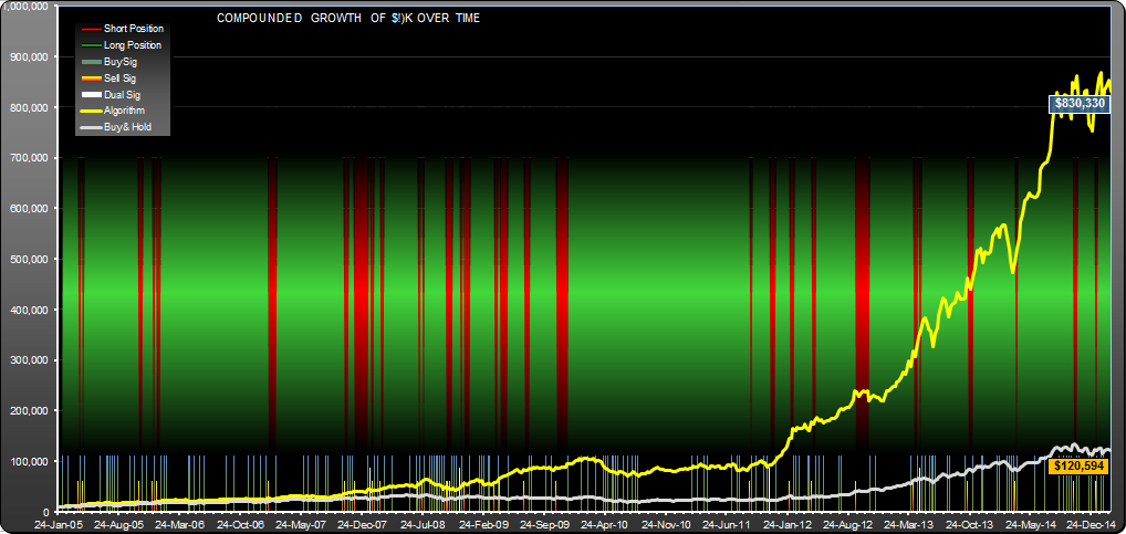
Note that the short side of the algorithm has a drawdown of 123%. If you look at the trades, you will see that this corresponds to a peak of $833,000 in Oct 90 and a trough of -$196,000 in May 91. This can happen on the short side of an algorithm, and would have led to expensive and quite possibly disastrous margin calls. The algorithm, however, recovered the following month when the stock price fell dramatically.  The long side of the algorithm made $1,066,052,956 with only $10K at risk.

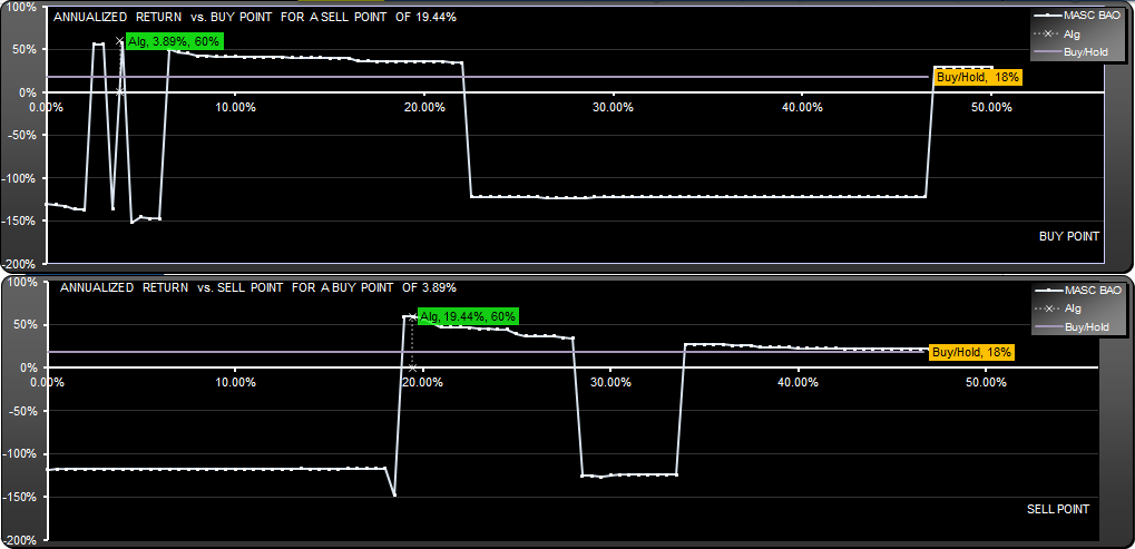
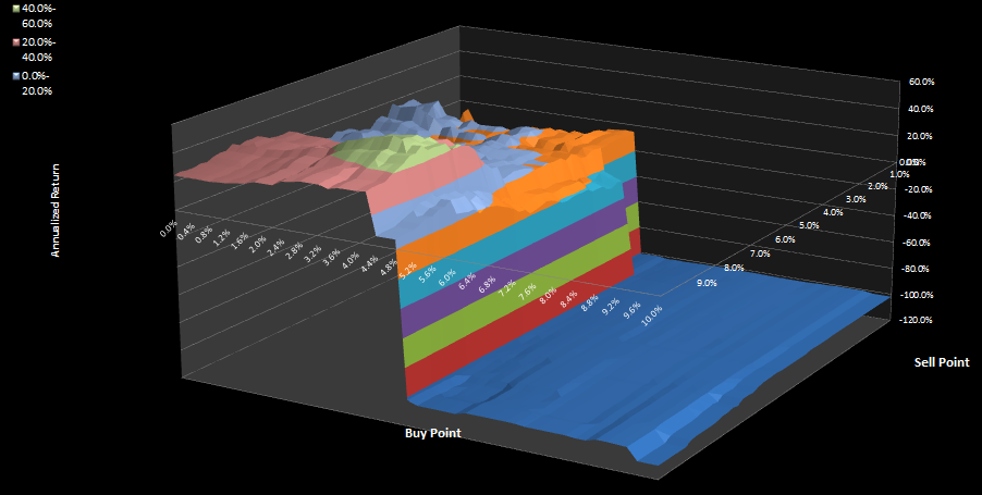
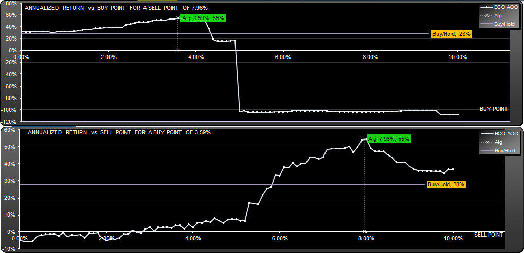
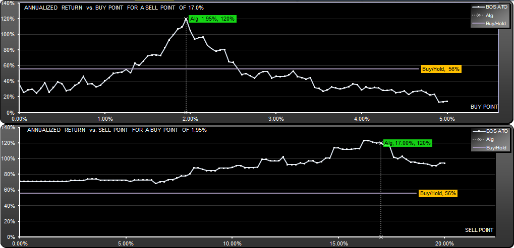
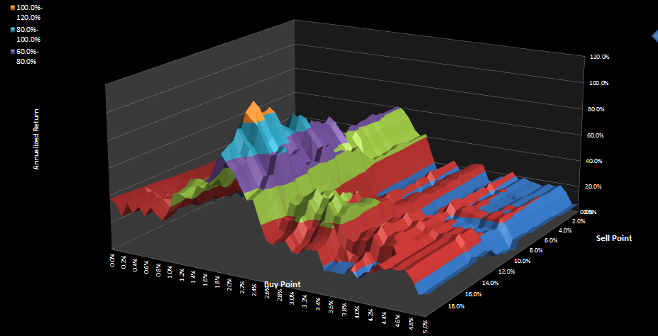
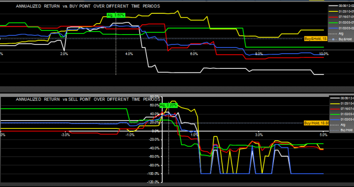
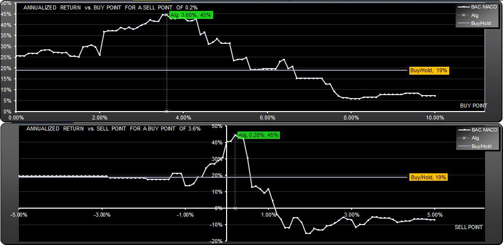
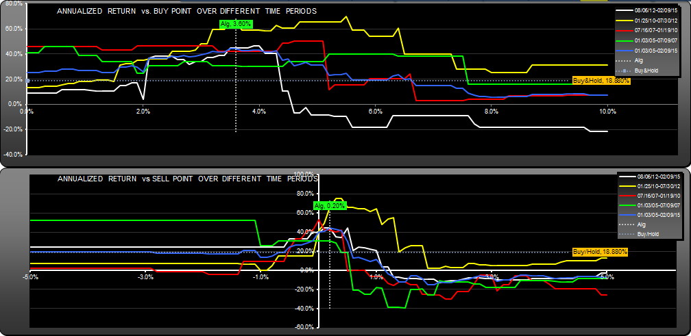
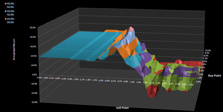
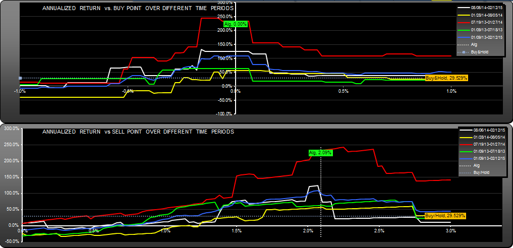
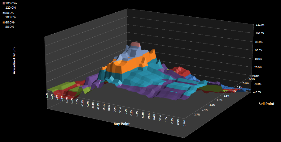
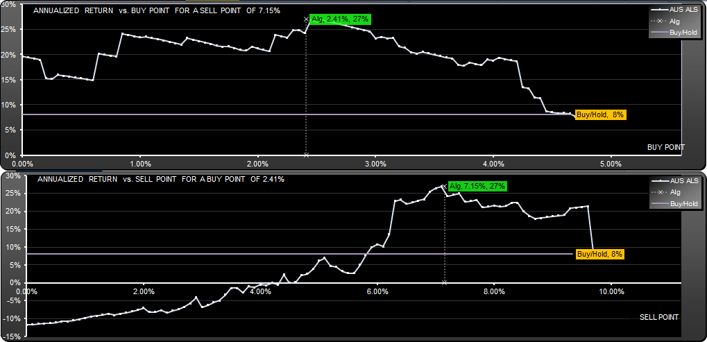
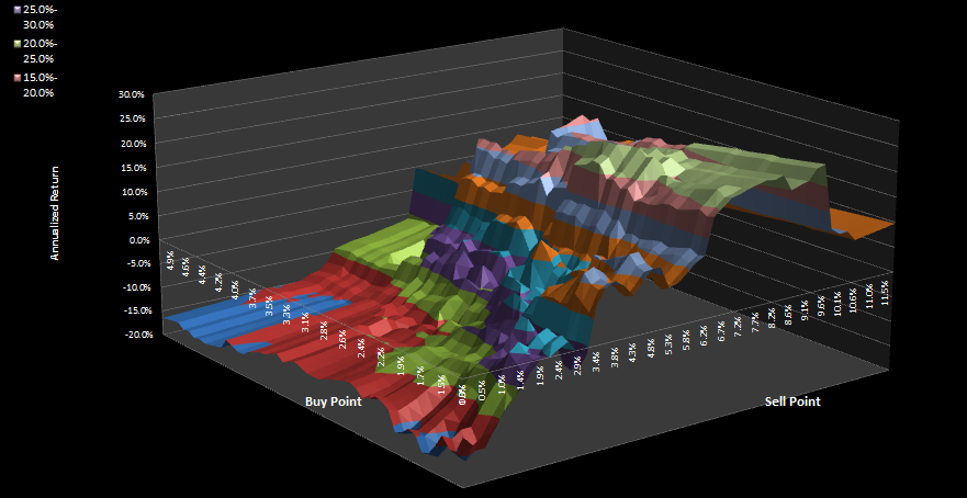
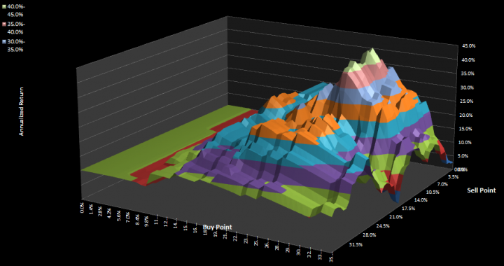
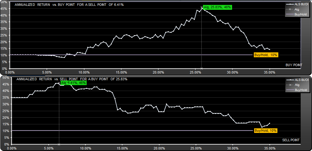
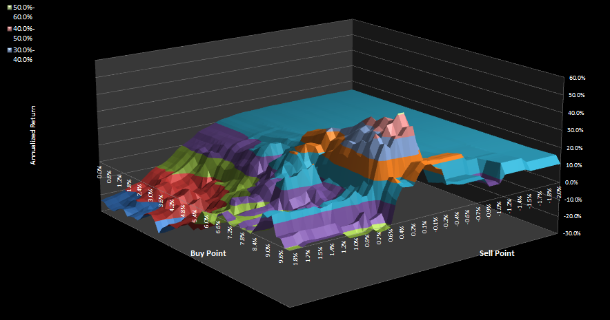
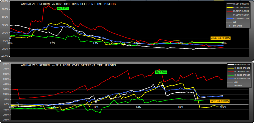
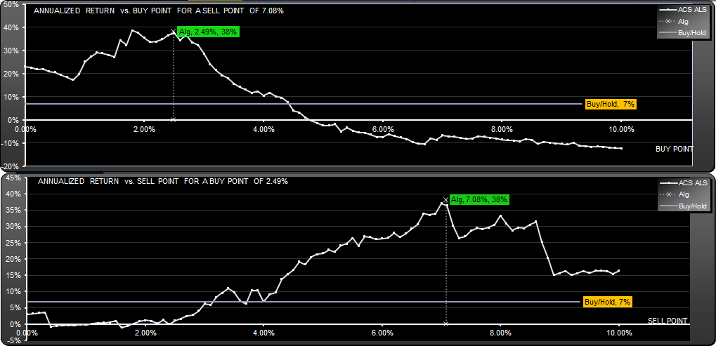
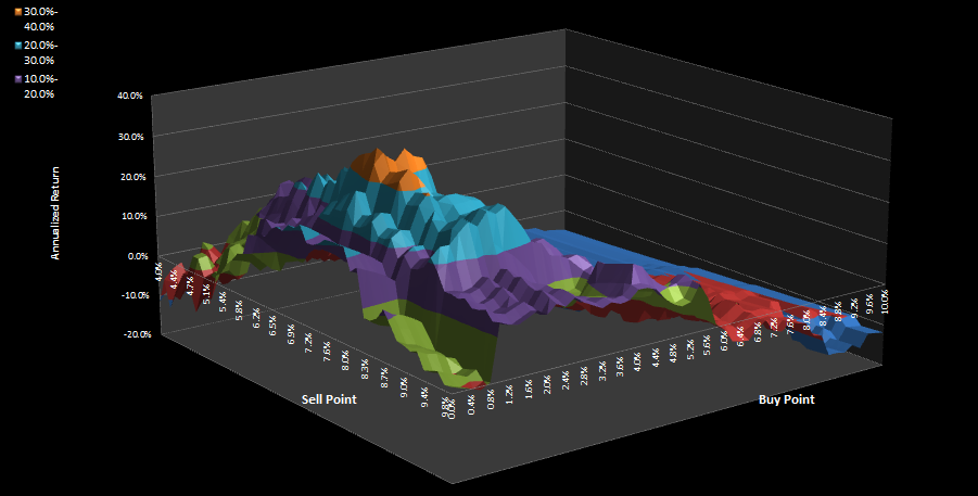
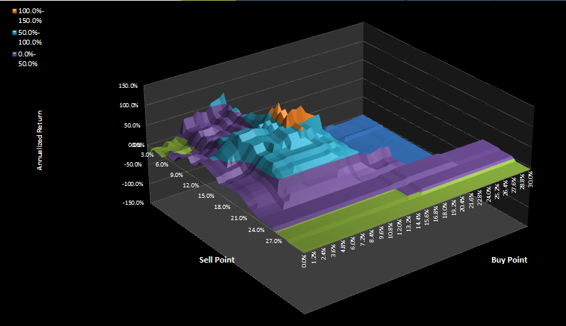
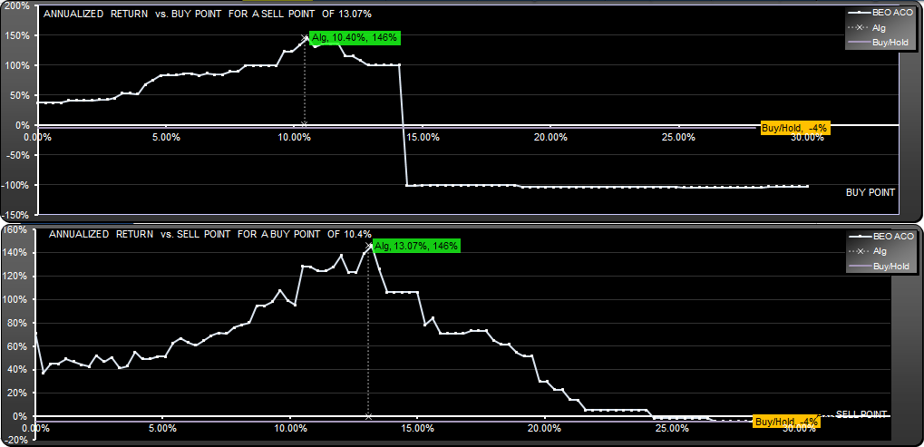
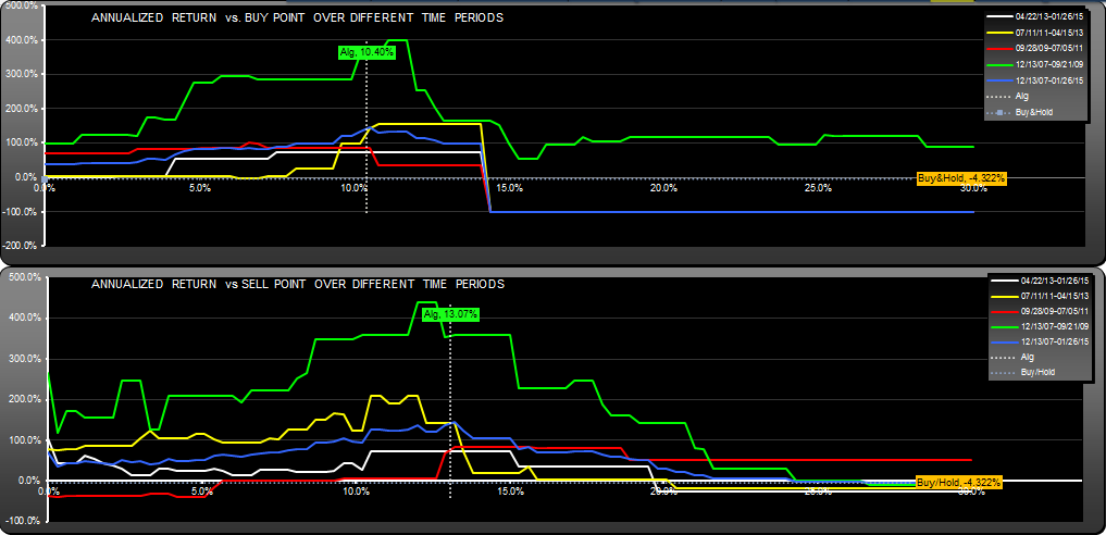
The scan shows how the return changes with choice of buy and sell point. We have chosen to show the peak, but better choices would have been in the center of the profitable regions.

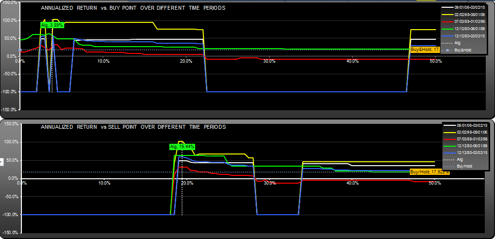
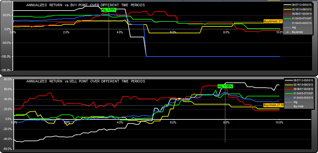
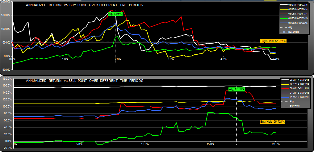
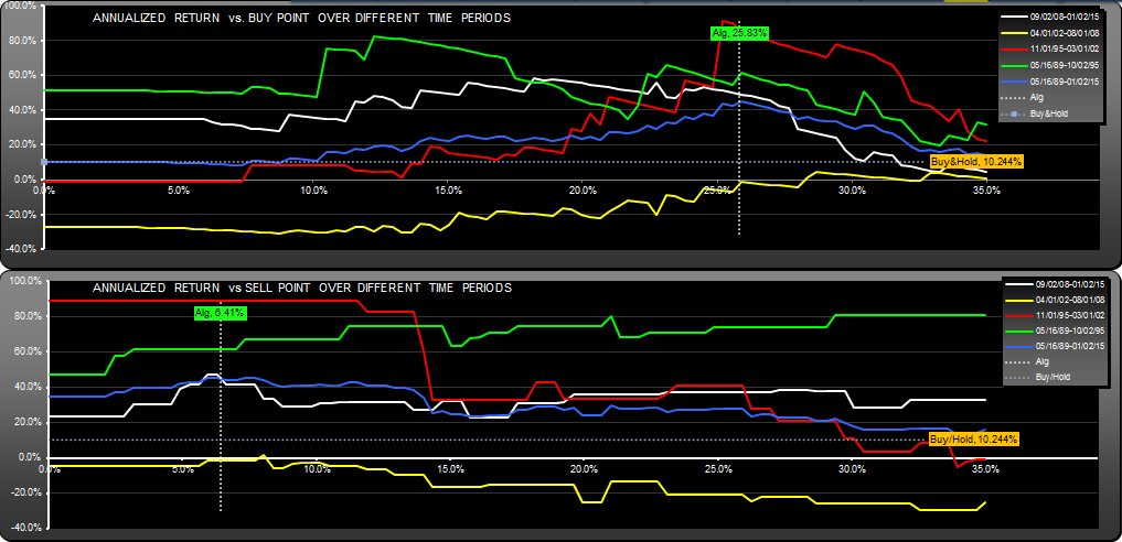
These scans show how returns change with buy/sell point for different timeframes.

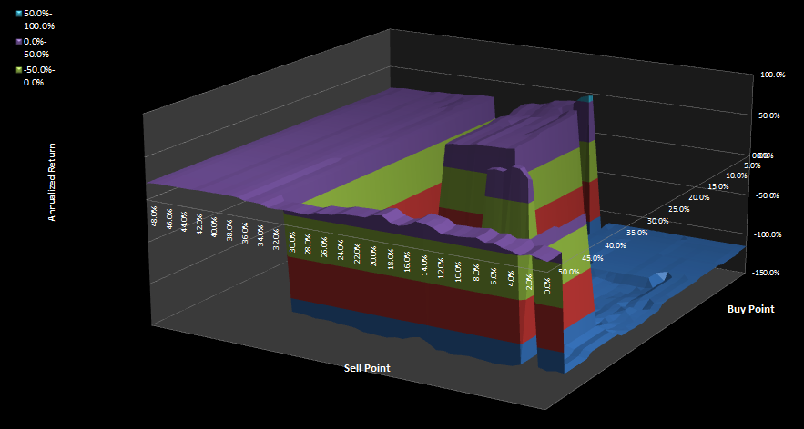
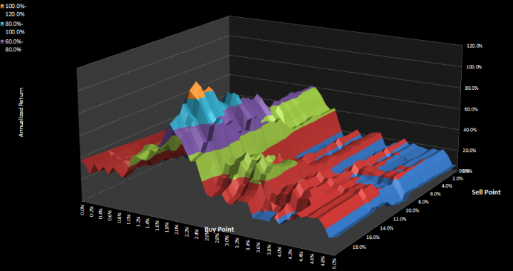
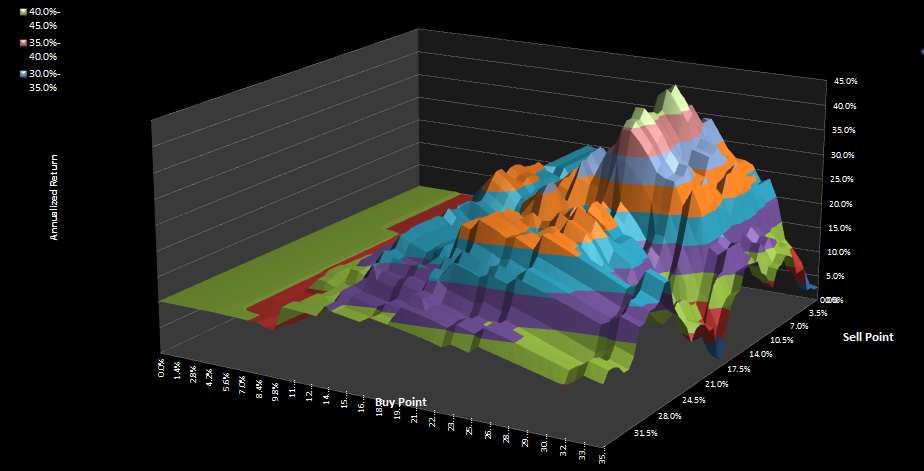
The scan shows returns for the entire buy/sell point space. High points are good, low points are, in this case, losses.

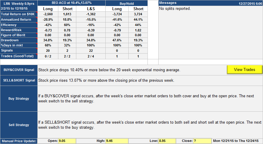
Please note that this post was edited 12/29/2105 to correct a calculation error on the short side of the algorithm.

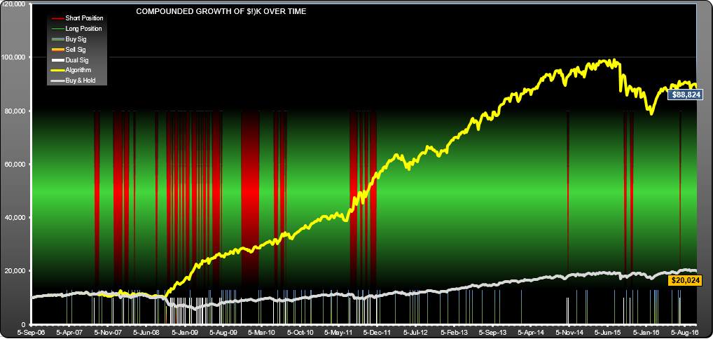
AAPL Apple Trading Strategy (Monthly) Update 10/20/2016

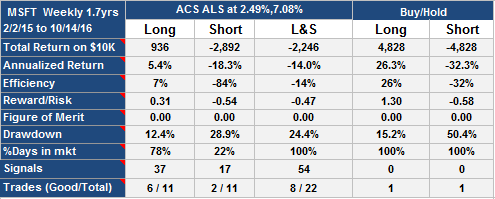
Strategy returned 11%, buy-hold -5%

AAPL Trading Strategy (M) Update 10/20/2016

AAPL Trading Strategy (M) Update 10/20/2016

AAPL Trading Strategy: Equity curve as of 10-20-2016

AAPL Trading Strategy: Equity curve as of 10-20-2016

GILD Trading Strategy (Weekly intervention)

This is a GILD trading strategy with weekly intervention required. I found algorithms with better returns, but they were less consistent over time and had more parameter sensitivity. I chose this one because of many favorable characteristics:-

  • Buy low, sell high type of algorithm, biased towards buying as befitting an upward trending stock like GILD.
  • Buy and sell at the weekly open was easy and convenient to implement
  • Buy and sell signals were well differentiated (only 4 dual signals) with good reinforcement on the buy side.
  • Good lifetime characteristics with each 2.5 year  period beating buy-hold.
  • 87% successful trades and a Sharpe Ratio of 2.03 vs 1.05 for buy-hold.
  • Gentle slopes on the parameter surface.

Note that charts were corrected 1-2-16 for an error in short-side return


Update 1-2-2016

GILD-W1 1-2-16 Update Table

Update 10/20/2016

GILD Weekly Trading Strategy Update Oct 20th 2016

GILD Weekly Trading Strategy Update Oct 20th 2016

PANW Trading Strategy (Daily Intervention)

This Palo Alto Networks PANW trading strategy would have given a 119% annualized return. Here, I chose to show only the long side of the algorithm because its more impressive than the short side (which only gave 27% annualized return). To appreciate the algorithm more, notice that the efficiency of the algorithm was close to 200%. Efficiency (as we define it) is the annualized return divided by the percentage of time you were in the market. Its the return you would have received if you had realized the same return all the time as you had got while you were in the market. The theory is that since you are not in the market all the time, you could have invested the money elsewhere.

Efficiency only applies to long or short style algorithms, since if you were running both long and short (L&S) you are in the market 100% and efficiency equals annualized return.

Updated 1-2-2016 to correct an error in the short-hold returns.

Update Aug 28th 2015:

PANW.D Update 8-28-15

Update 2-1-2016

Algorithm has had better return, efficiency and drawdown than Buy/Hold, but not consistently. Optimum buy point dropped to 1.25% (which would have given a return of $4,316)

PANW-D Update 1-2-16


Update 10-10-2016

Algorithm continues to have better return, efficiency and drawdown than Buy/Hold. Buy-hold lost 12% annualized, this strategy made 28.7% annualized. Efficiency (55%) is what the strategy would have made annualized, had the money been invested at the same rate while the strategy was out of the market.

PANW Trading Strategy Performance since publication as of Oct 10th 2016

PANW Trading Strategy Performance since publication as of Oct 10th 2016

Here is a view of the performance since original publication in March 2015:

PANW Trading Strategy, performance since initial publication, 60% gain vs 12.3% for buy-hold

PANW Trading Strategy, performance since initial publication, 60% gain vs 12.3% for buy-hold.

GOOGL Trading Strategy (Weekly Setup)

Algorithm for GOOGL based on monthly OHLC data and requiring monthly setup.

GOOGL.M Time

Buy signals around 3 times more frequent than sell signals, some overlap (dual signal months shown as white lines). 80% long, 20% short. Algorithm showing flattening out of performance in recent months.

GOOGL.M Table

GOOGL.M Performance table and strategy description. Showed about 3 times the reward-risk of buy-hold. Strong bias to buy side (as is appropriate for upward trending stocks), clearly shown in signal count and %days long vs. short.

GOOGL.M Scan

Return vs. parameter for buy and sell parameters. Buy side is reasonably insensitive. Sell side seems more highly tuned, however algorithms of the "misses target" type often have this characteristic of being tightly clustered around zero.

GOOGL.M Life

The life chart shows parameter sensitivity for different time periods. All timeframes beat buy-hold by a decent margin.

GOOGL.M Surface

GOOGL Surface chart showing how return changed with buy and sell parameters.


Update 10/20/2016

GOOGL Trading Strategy Weekly Update Oct 19th 2016

GOOGL Trading Strategy Weekly Update Oct 19th 2016

MSFT Trading Strategy (Daily)

Here is a strategy that worked on MSFT for the last 2 years. It gave returns around five times better than buy-hold, a total return of 360% vs. 70% for buy-hold. Drawdown was 10.6% vs. 17.9% for buy-hold. Backtest results are shown in the graphs below.

MSFT daily trading strategy

MSFT daily trading strategy, performance table and strategy details. Note that "user defined price" is the average of the high and low of previous day and the open of current day [ (h+l+o)/3 ]. A few observations; return and reward/risk was 5x better than buy-hold. Drawdown of 10.6% vs. 17.9% for buy-hold. Long side worked much better than short side.

MSFT daily strategy, graph showing how return varied with buy and sell point parameters for different time periods. The blue line shows the overall 2 year graphs, the others are for 6 month periods. All periods gave better returns than buy-hold. Note that buy point range is fairly restricted.

MSFT daily strategy, surface plot of return (z axis) as it changes with buy and sell point. The blue plateau is roughly the same return as buy-hold.

On Jan-5-2016 this post was corrected for a short-side return error, and a commission of $7 per trade was factored in.

Update Jan 5th 2016

This algorithm was not a stellar performer. Since publication it has been essentially flat, let down badly by the short-side performance

MSFD-D Table Update Jan-5-2016

To be fair, the long side performance was reasonable, but buy-hold was on a roll.

Optimum parameters for this period were different than the original posting, buy point -0.98%, sell point 10.33% for this result:

MSFD-D Table Update Jan-5-2016 Optima

Again, long-side was much more interesting than short-side performance.

Update Oct 19th 2016

This algorithm continues to perform badly

MSFT Trading Strategy (Daily) update Oct 19th 2016

MSFT Trading Strategy (Daily) update Oct 19th 2016


SPY Trading Strategy (Weekly)

Shows the results of backtesting a trading strategy for the stock SPY (SPDR S&P 500 ETF) over the 10 year period 1/18/05 to 2/23/15. This was a weekly strategy meaning that it needed setting up once a week, and it traded once a week or less. I chose this strategy because it gave the best total return (1020% vs 120% for buy-hold), not because of its longevity characteristics which are not superlative. That said, it was reasonably well behaved, staying long in the run up to the 2009 crisis, going mostly short then essentially staying long since 2011. It also displayed a good tolerance to changes in the buy and sell points.

Note that this was a buy high, sell high strategy; a sell signal was (with one exception) always accompanied by a buy signal in the same week, but since each week you were following either the buy or the sell strategy, there was never two trades in a week. There were a total of 118 buy signals and 43 sell signals.

Please note, this post was edited Jan 6th 2016 to correct an error in the short-side calculations.

Trading strategy for SPY with a weekly setup. The strategy (yellow line) returned $102,005 over a 10 year period for a $10K initial investment. Buy and hold returned $11,846. Trading signals were reinforcing--note that every week with a sell signal also had a buy signal.

SPY Weekly, tabular view of the backtest. Trading strategy gave 27% annualized return vs. 8% for buy-hold. Reward/risk was around 7x better for the strategy. Note that the "user defined" referred to in the buy signal is the average of the current weeks open price, the previous week's high and the previous week's low. Also of note, drawdown was only 21.3% (Sept '08) vs. 55.3% for buy-hold (March '09).

Charts show how annualized return varies with buy/sell point (for a fixed sell/buy point). For a sell point of 7.15% all buy points 0-6.5% were profitable. For a buy point of 2.41%, all sell points in the range 4.1%-9.6% were profitable.

This chart shows return of the algorithm for different time periods, and how they change with buy and sell point. The green line (1/05 to 7/07) shows little improvement over buy-hold. The white line (8/12 to present) is distinctly lower showing a tailing off in performance in recent times. In fact, the algorithm has sub-performed buy-hold for the last 3 years, by a small margin. You can see from the time chart that the algorithm has stayed mostly long for 3 years. Some may like this behavior; an algorithm that stays largely out of the way in the good times. Others may argue that the algorithm fails to exploit recent price fluctuations.

SPY weekly, surface plot. Shows how return varies with changing buy and sell point percentages. The area of interest is the plateau. It is wide with few cliffs which is what you want to see.

Update Jan 6th 2016

This algorithm began to break down around Aug 10th. Since publication it has lost around 16%.

SPY-W Table Update 1-6-2016

SPY-W Equity Update 1-6-2016

Update Oct 19th 2016

Still unspectacular performance from this:

SPY Trading Strategy (Weekly), Update 10-19-2016

SPY Trading Strategy (Weekly), Update 10-19-2016

SPY Trading Strategy (Weekly) Update Oct 19 2016 Equity

SPY Trading Strategy (Weekly) Update Oct 19 2016 Equity

MU Trading Strategy (Monthly)

Micron Technologies monthly trading strategy, 46% Annualized Return, 25 years

Please note, this post was edited Jan 6th 2016 to correct an error in the short-side calculations. The original post showed an annualized return of 57%, which was erroneous. Below are shown the corrected results for this algorithm.

Micron Technology (MU) trading strategy base on monthly OHLC data. Would have returned $153,063,510 for a $10K initial investment. B/H returned $111,745 over the same period (5/16/89 to 2/2/15). Signals (at bottom of graph) generally show good reinforcement with occasional periods of confusion. Background red/green stripes show short/long hold periods

MU Monthly. Annualized return for this trading strategy was 46% vs 10.2% for buy/hold. Drawdown was a disconcerting 97.1% for buy/hold in Dec 2009, vs. 57% in Sept 2006 for the trading strategy. The price jumps reported were 50% drops in '87 and '00. The "user defined price" referred to in the strategy is the open price of the current month plus the high and low price of the previous month, divided by 3. Reward-risk was 6.7 times better than B/H using return/drawdown+10% as the yardstick.

This graph shows the effect of changing the buy and sell parameters on the annualized return of the algorithm. For a buy point of 25.83%, all sell points 0 through 35% were profitable. For a sell point of 6.41%, all buy points 0 through 35% were profitable.

The life graph shows the return vs buy/sell points for different periods. The problem here is that the yellow graph shows that there was a period (5/89 to 10/95) with much worse return than the other periods. A more consistent algorithm over time would be preferable to the author, even if it had lower returns.

The parameter surface shows how the return changed over the whole parameter space. Cliffs and steep slopes are not good, but for this the drop-offs are reasonable.


MU Monthly, Update Jan 6th 2016

MU-M Table 1-6-2016

Since original publication, this algorithm would have returned 58%

MU-M Equity 1-6-2016

MU Monthly Trading System, Update 10/19/2016

The strategy, since publication in Feb 2015, has performed much better (86% return) than buy-hold and short-hold, with good drawdown. However, the optimum buy parameter for the period (16.45%) would have yielded a 151% return.

MU Monthly trading strategy update 10/192016

MU Monthly trading strategy update 10/192016

Since 5/16/89 the strategy would have returned $279,572,374

WMT Daily. For a $10,000 investment, buy and hold returned $3,280. The trading strategy detailed here returned $13,632 over the period 1/8/13 to 2/11/15.

WMT Trading System (Daily)

For the period 1/8/13 to 2/11/15 the trading strategy returned $13,608 on an initial investment of $10,000. Buy and hold returned $3280. At the bottom of the graph are the signals. In this case the buy signals show good reinforcement, generally a buy signal is followed by several other buy signals. Sell signals show little reinforcement. Red and green bands show when the stocks were held long (green) or short (red).

WMT Daily. The tables show the annualized return of the trading strategy (50.8%) vs. buy and hold (14.7%) for the 2 year period 1/8/13 to 2/11/15. Drawdown was 6.2% vs. 10.5% for buy-hold. You can also see how you would have fared going only Long or Short or short-and-hold. The lower table describes the signals and the strategy in detail. The Long and Short strategy is described which requires holding the stock long or short at all times, however you would also have made a profit taking just the long or short side.

These graphs show how the return varies with changing the parameters of the algorithm. Note that for a sell point of 0%, all buy points to beyond 10% were profitable. However the algorithm was highly sensitive to changing the sell point, which had to be between 0% and 0.5% to give significantly advantageous returns. If outside of this narrow range, the algorithm was only as good as buy-hold.

The Life graphs show how the returns look over four different time periods. In general it is best to look for systems with consistent returns. For this strategy, all four time periods showed returns better than buy-hold.

WMD Daily. This shows how the return varied when the buy and sell points were varied. Notice the sell point range is much narrower that the buy point range. The algorithm only worked for a very small range of sell points.

Update Jan 9th 2016

WMT-D Table 1-9-16

Since original publication, the algorithm like the underlying stock has done poorly.


Update 10/19/2016

WMT Daily Trading Strategy Update 2016-10-19

WMT Daily Trading Strategy Update 2016-10-19

MSFT Trading System (Weekly)

This graph shows the equity curve of the trading system for Microsoft (MSFT) over a ten year period, 1/3/05 to 2/6/15 for a $10K initial investment. The value increased to $262,144 vs. $19,521 for buy-hold. The background bands show if the stock was held long (green) or short (red). Note that most of the sell signals (shown at the bottom) are also dual signals as a buy signal generally occurs in the same time period. This is common with this kind of trading strategy.

The trading strategy works off weekly data, so it trades at most once a week and uses stop cover/buys and limit short/sells. The L&S column shows results for trading both Long and Short. Drawdown (20%) was much better than for buy-hold (57%).

Here we compare the returns over different time periods, as they change with buy and sell point. We look for algorithms which give consistent returns–this one has one period of high returns (the red lines) and a period of returns similar to buy-hold (the green lines). Overall the returns were good (the blue lines).

Plotting how returns change with buy and sell points gives us an idea how sensitive the algorithms are to changes in parameters. Here we see two broad peaks indicating that the algorithms are not overly sensitive to changes in parameters. In fact this buy point was profitable for all values of sell point from 2.5% to 10%.

In the surface plot of return vs. buypoint/sellpoint we are looking for high ground, not too close to cliffs or valleys. For this algorithm there is a distinct hill feature showing a fairly stable exploit region.

Looking at 100 week performance for the same algorithm shows an improvement over buy-hold and better drawdown, although the equity curve (below) is similar.


Update 10/19/2016

This strategy has lost around 22% since inception, the underlying stock has gained 48%.

msft-w-table-update-20161019

LRN Trading Strategy (Weekly)

K12 Inc (LRN)

LRN.W Equity Corr

LRN.W Table Corr

LRN.W Surface Corr

LRN.W Scan Corr

LRN.W Life Corr

Update 12/27/2015

The above plots have been corrected for an error in the short side calculations. Below are updated equity curves and tables up until Dec 2015. The algorithm lost 13.6% over this time. The underlying stock dropped by 37.2%.

LRN.W Equity Update Dec15

LRN.W Table Update Dec15

LRN Table Update2 Dec15

LRN.W Equity Update2 Dec15


Update 10/19/2016

Since first publication in Feb 2015, this strategy has outperformed both buy-hold and short-hold. Here are the performance table and equity curve for the period since publication:

LRN Trading Strategy Update

LRN Trading Strategy Update


LRN Trading Strategy, Update 10/19/2016

LRN Trading Strategy Equity Since Inception

LRN Trading Strategy Equity Since Inception

lrn-w-update-20161019-table-since-inception