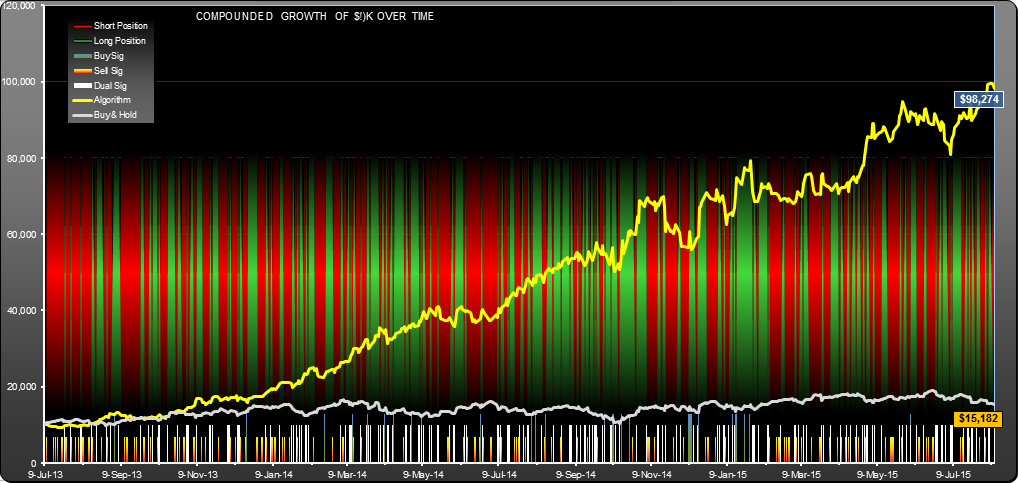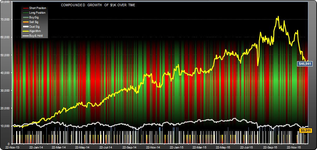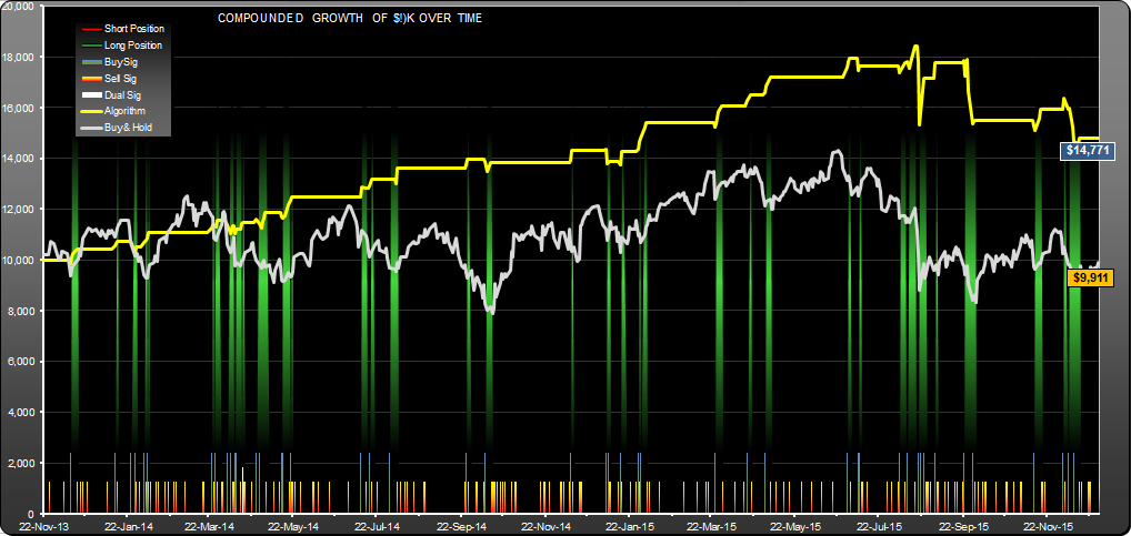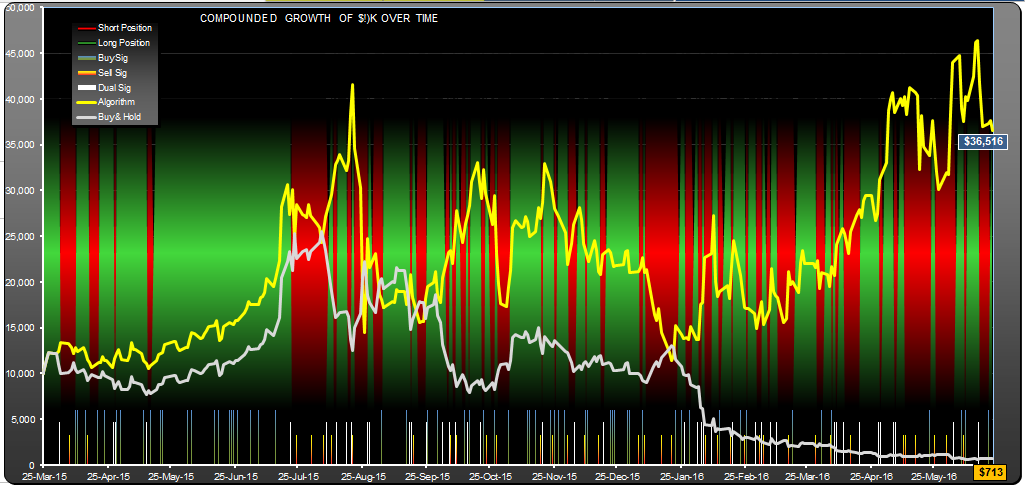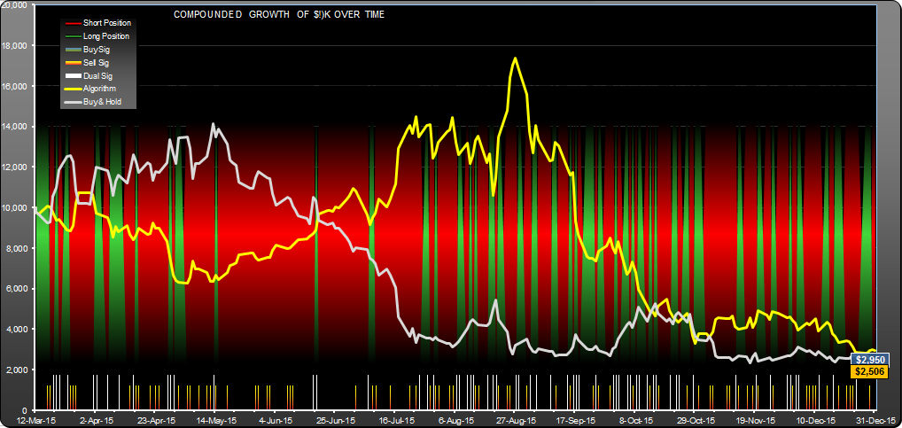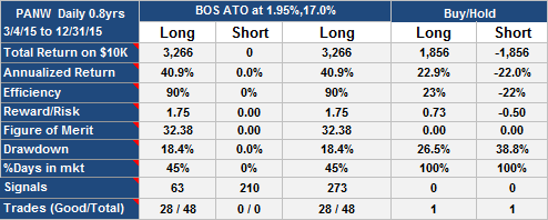
GLD is the much traded SPDR Gold Trust ETF. I find these two GLD trading strategies interesting because they gave reasonable results (32.6% and 48% annualized return) for each of the four 6 month periods of the analysis. The strategies require daily intervention.
Strategy 1: BCS AHC
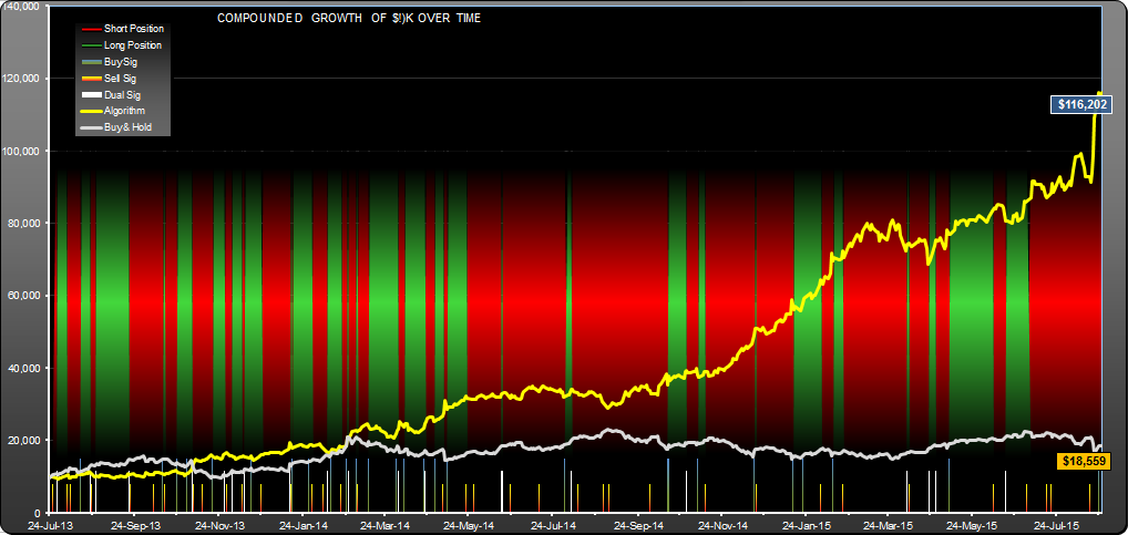
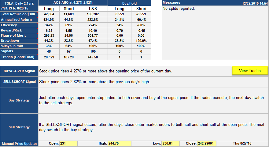
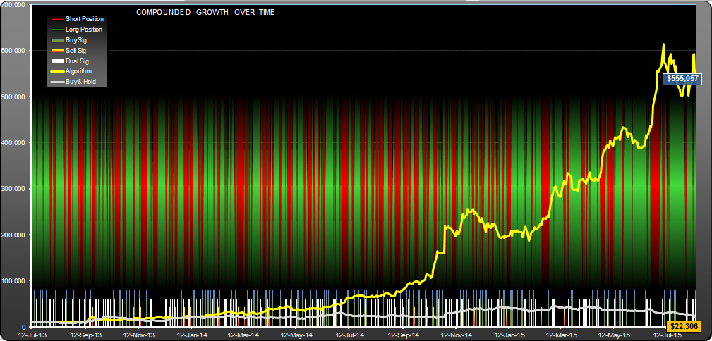
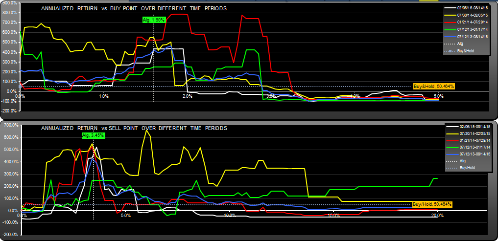
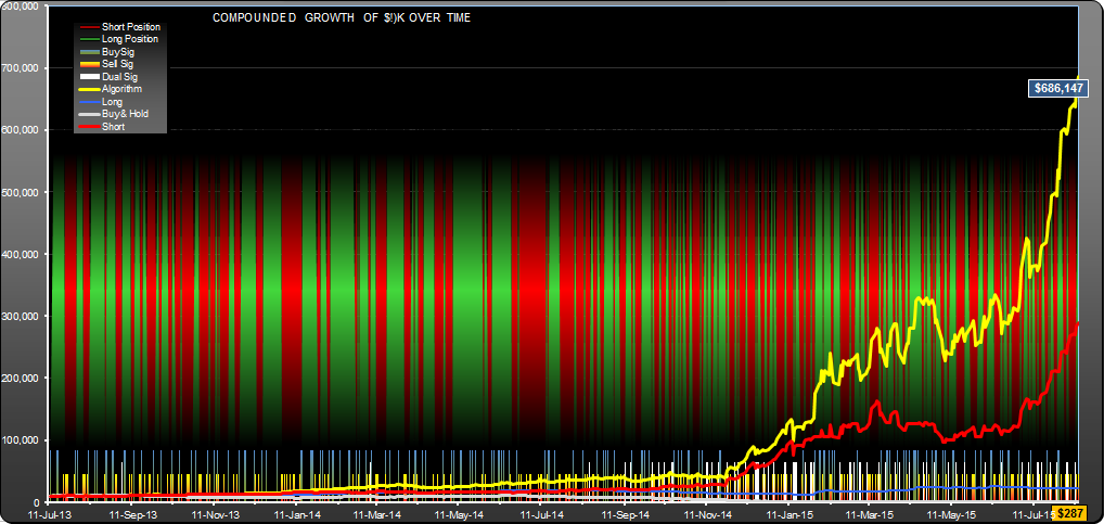
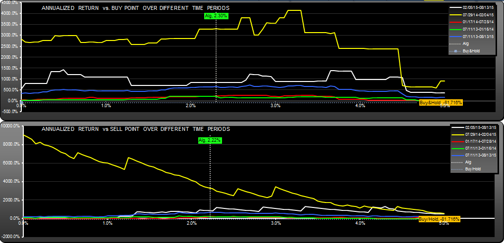
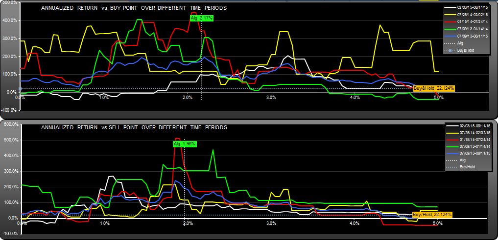
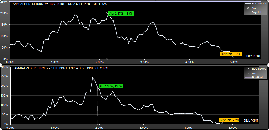
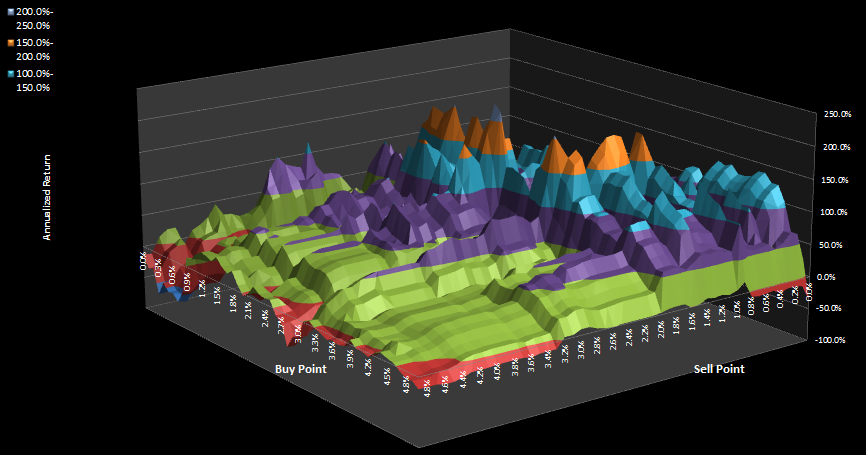
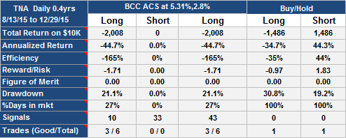
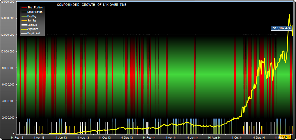
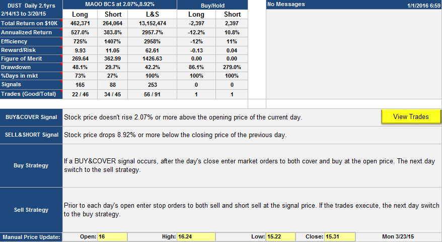
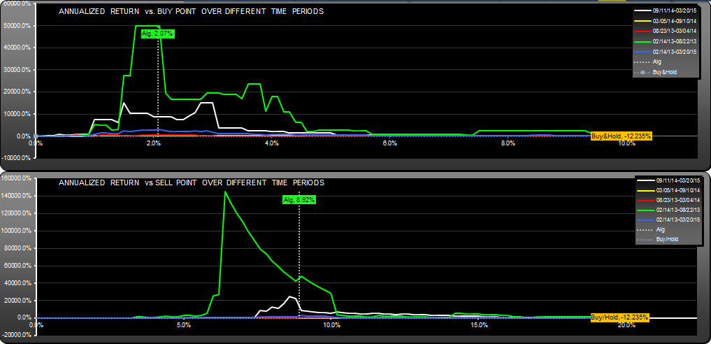
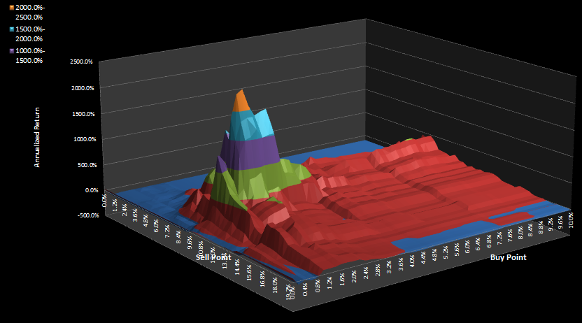
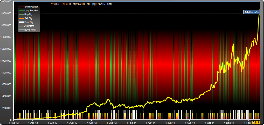
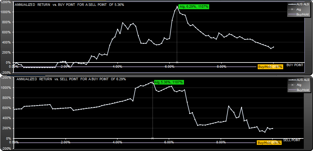
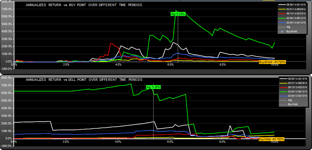
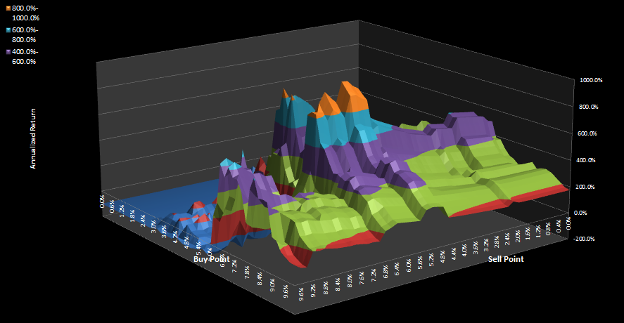
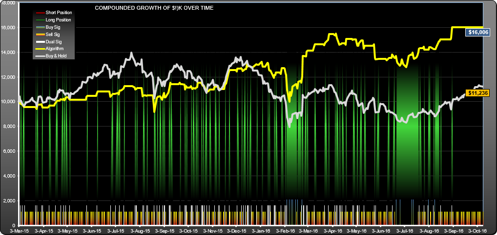
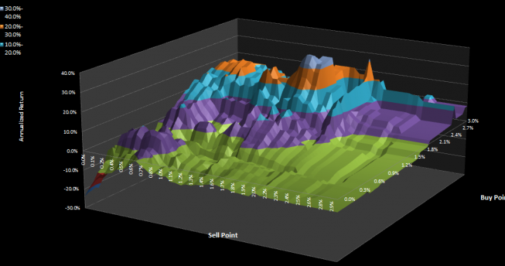
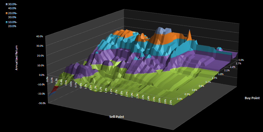
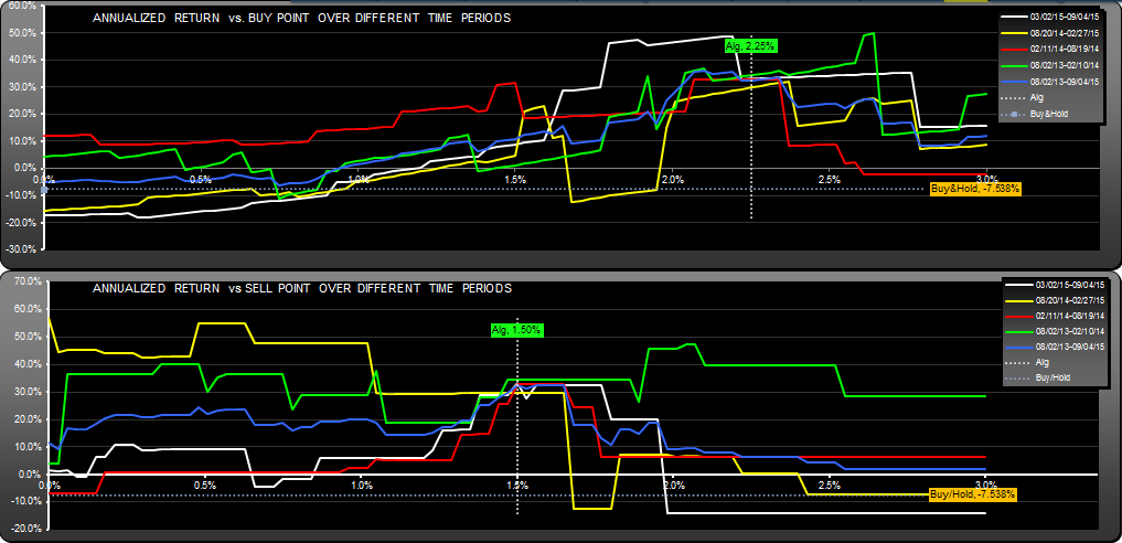
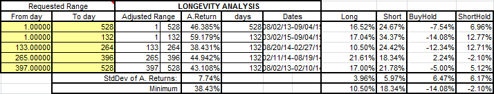
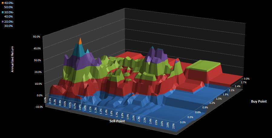
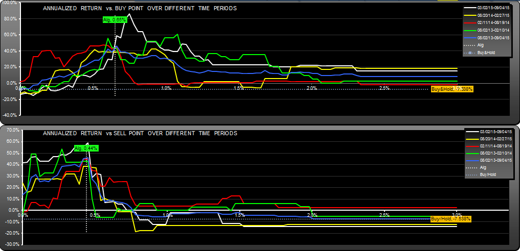
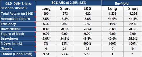
This is a buy on fall, sell on rise strategy using the close price as the buy reference and the high price as the sell reference. As you can see from the life chart and the longevity analysis, the lowest return for the last four 6 month periods was close to 30% annualized. You can easily find algorithms with over 50% annualized return for GLD, but they are not as consistent, with lowest quartus returns of around 14%.
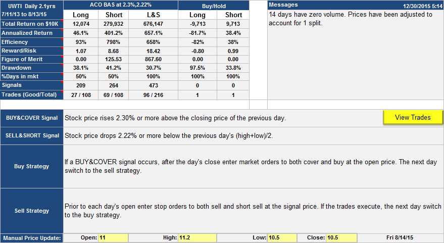
I would prefer to see more reinforcement on the signals, but there it is. As of Sat Sept 5th, this strategy is Short with no transactions pending.
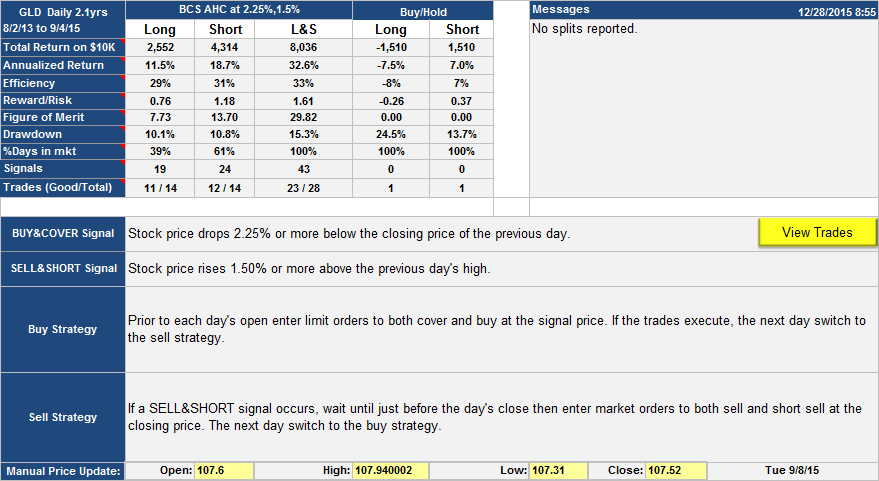


You can view the trades in spreadsheet format here: GLD.D Trades
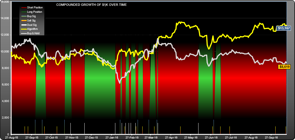
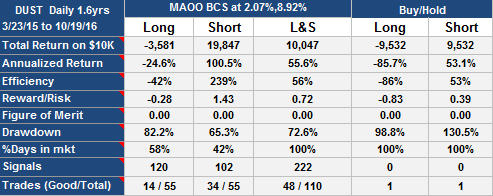
Strategy 2: AOO AHCI
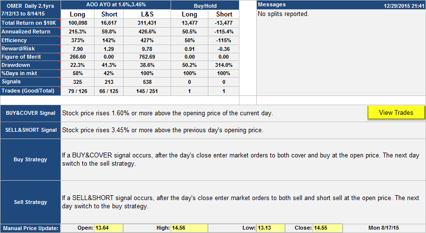
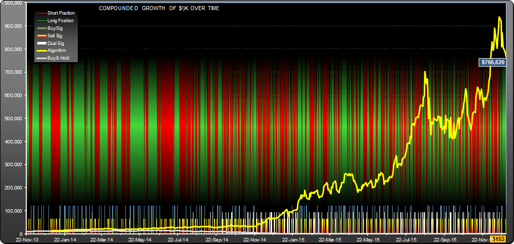
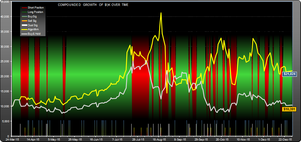
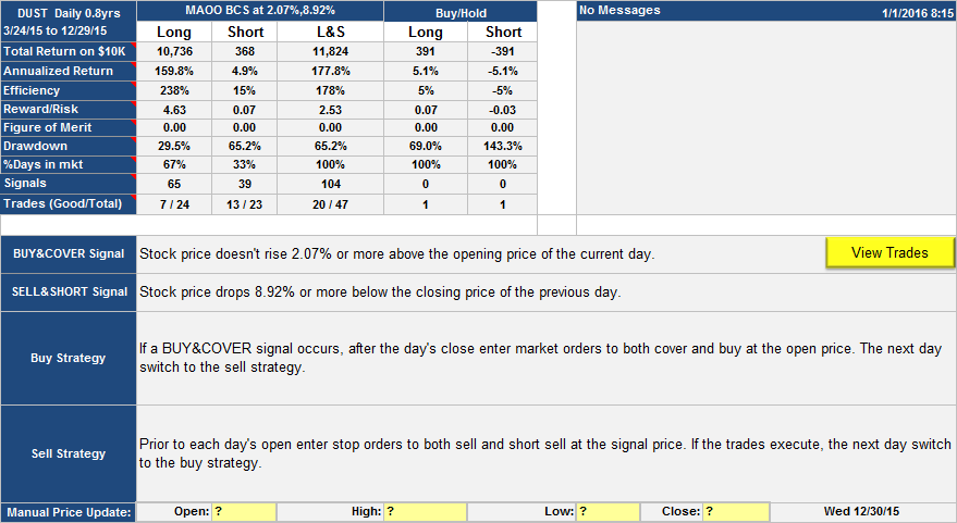
In many ways this strategy shows better results than the BCS AHC strategy, for example there was lower drawdown, higher return, better signal reinforcement and good consistency (minimum 6 month quartus return of 38.43%). On the other hand, signals were cluttered, with 67 dual signal days, 50 buy signal days and 75 sell signal days. Also, its not an trading strategy that makes intuitive sense; buy on rise, sell on rise. Maybe it is one of those serendipitous occurrences, we shall see. Notice the sell strategy is almost the same as for BCS AHC but the sell signal percentage is quite different.
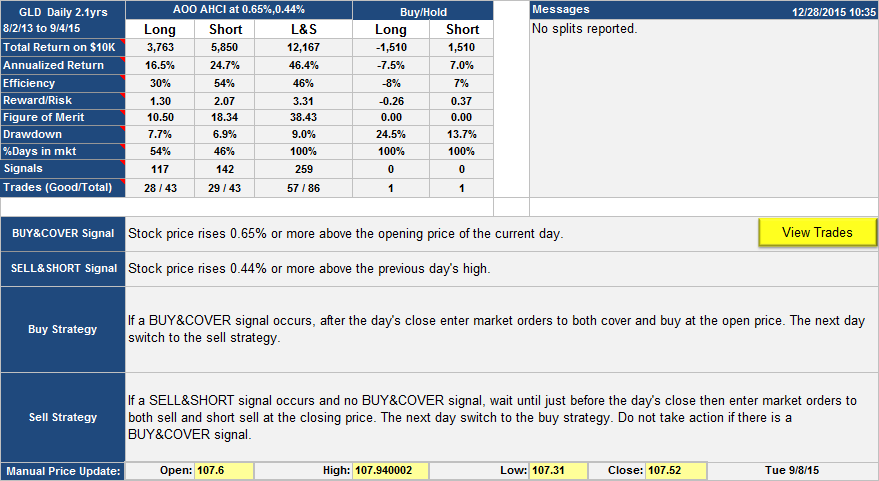

As of Sat Sept 5th, the strategy is Short with no transactions pending. For a list of trades in Excel format: GLD.D2 Trades. For a more detailed explanation of the above charts, please go here.
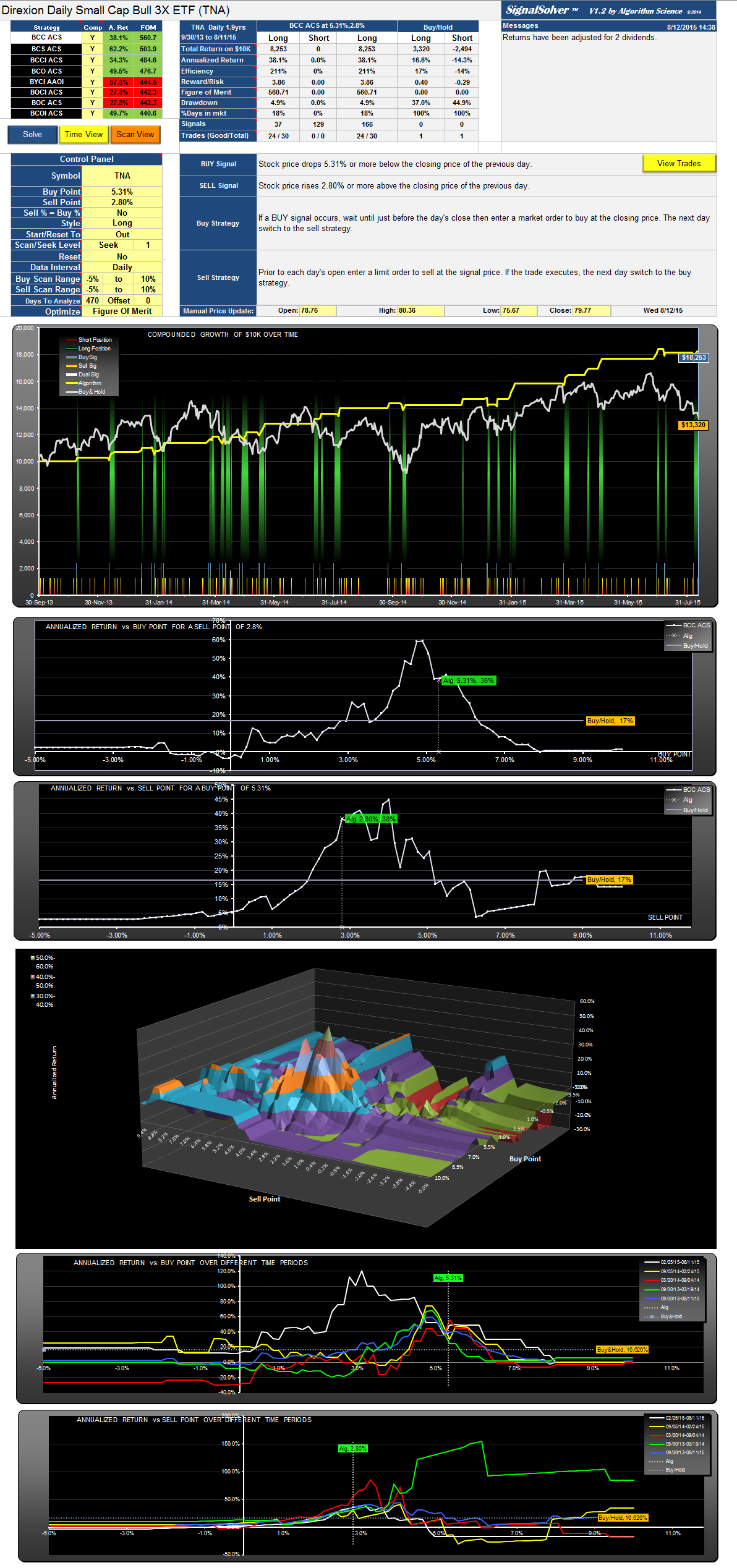
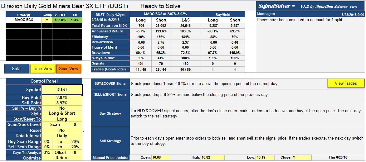
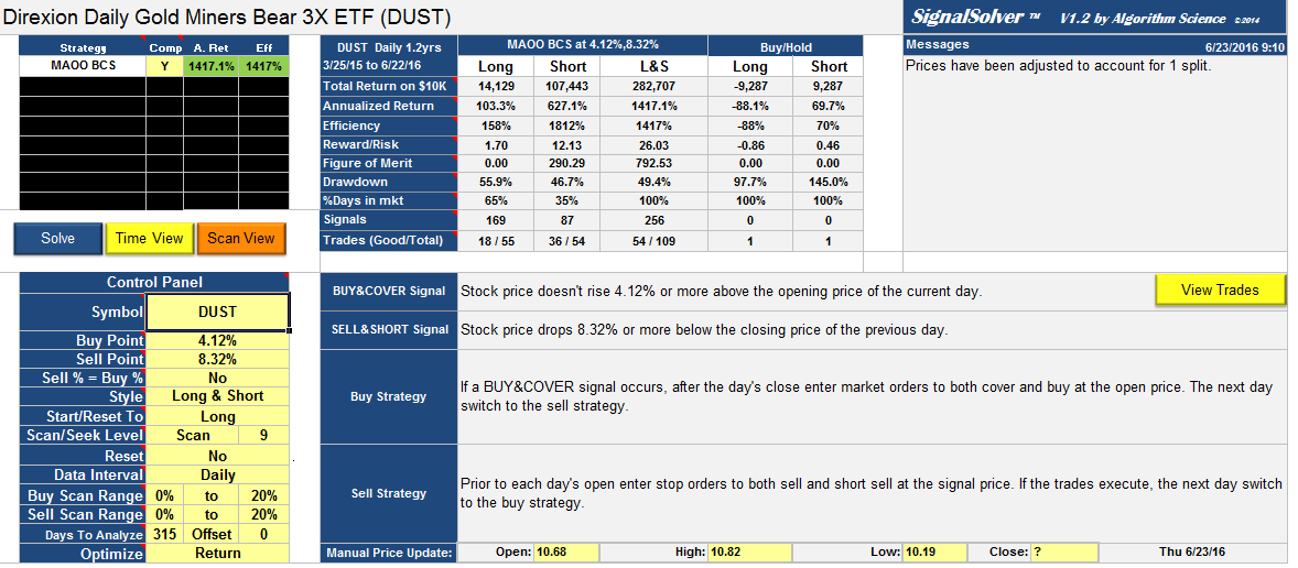
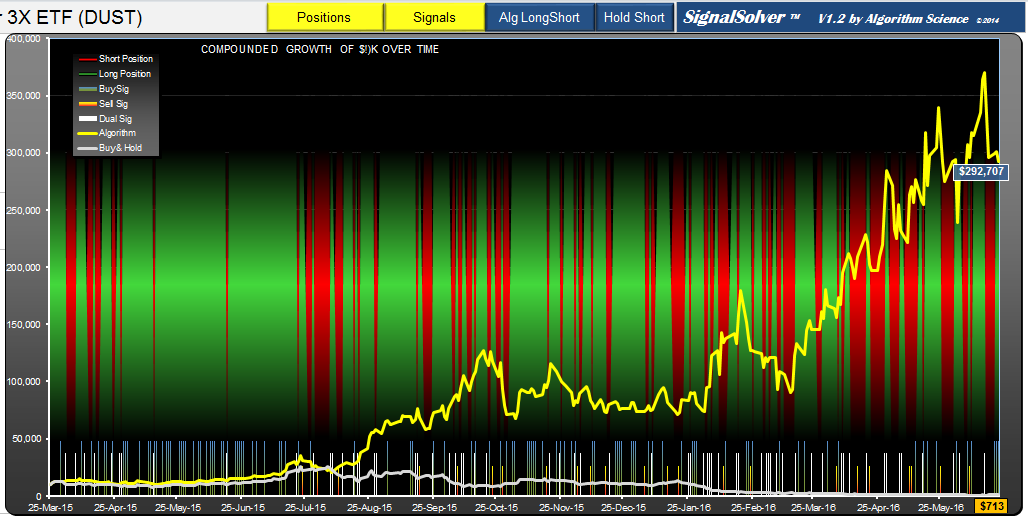
Algorithms were discovered by SignalSolver.
Please note, the above analysis was corrected on 12/28/2015 to reflect a bug fix in SignalSolver. Original returns were $9530 and $12753 respectively.
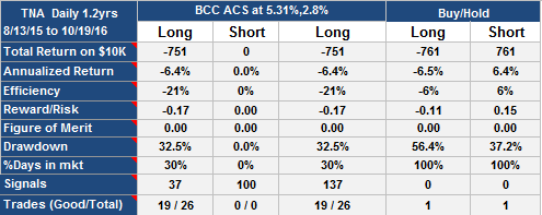
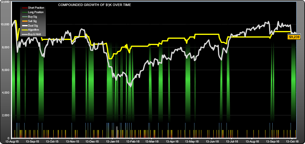
Update Oct 21st 2016
Both algorithms peaked 12/30/2015.

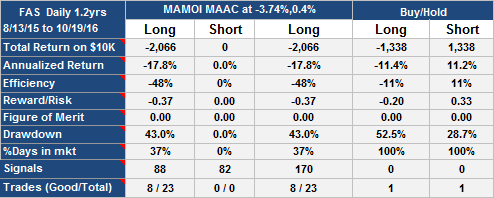
GLD Trading Strategy AOO AHCI Update Oct 21st 2016
GLD Trading Strategy BCS AHC Update Oct 21st 2016